the Creative Commons Attribution 4.0 License.
the Creative Commons Attribution 4.0 License.
 | 26 Jun 2018
Modelling feedbacks between human and natural processes in the land system
Alan Di Vittorio
Peter Alexander
Almut Arneth
C. Michael Barton
Daniel G. Brown
Albert Kettner
Carsten Lemmen
Brian C. O'Neill
Marco Janssen
Thomas A. M. Pugh
Sam S. Rabin
Mark Rounsevell
James P. Syvitski
Isaac Ullah
Peter H. Verburg
The unprecedented use of Earth's resources by humans, in combination with increasing natural variability in natural processes over the past century, is affecting the evolution of the Earth system. To better understand natural processes and their potential future trajectories requires improved integration with and quantification of human processes. Similarly, to mitigate risk and facilitate socio-economic development requires a better understanding of how the natural system (e.g. climate variability and change, extreme weather events, and processes affecting soil fertility) affects human processes. Our understanding of these interactions and feedback between human and natural systems has been formalized through a variety of modelling approaches. However, a common conceptual framework or set of guidelines to model human–natural-system feedbacks is lacking. The presented research lays out a conceptual framework that includes representing model coupling configuration in combination with the frequency of interaction and coordination of communication between coupled models. Four different approaches used to couple representations of the human and natural system are presented in relation to this framework, which vary in the processes represented and in the scale of their application. From the development and experience associated with the four models of coupled human–natural systems, the following eight lessons were identified that if taken into account by future coupled human–natural-systems model developments may increase their success: (1) leverage the power of sensitivity analysis with models, (2) remember modelling is an iterative process, (3) create a common language, (4) make code open-access, (5) ensure consistency, (6) reconcile spatio-temporal mismatch, (7) construct homogeneous units, and (8) incorporating feedback increases non-linearity and variability. Following a discussion of feedbacks, a way forward to expedite model coupling and increase the longevity and interoperability of models is given, which suggests the use of a wrapper container software, a standardized applications programming interface (API), the incorporation of standard names, the mitigation of sunk costs by creating interfaces to multiple coupling frameworks, and the adoption of reproducible workflow environments to wire the pieces together.


Models designed to improve our understanding of human–environment interactions simulate interdependent processes that link human activities and natural processes but usually with a focus on the human or natural system. When simulating the land system, such models tend to incorporate either detailed decision-making algorithms with simplified ecosystem responses (e.g. land-use models) or simple mechanisms to drive land-cover patterns that affect detailed environmental processes (e.g. ecosystem models). These one-sided approaches are prone to generating biased results, which can be improved by capturing the feedbacks between human and natural processes (Verburg, 2006; Evans et al., 2013; Rounsevell et al., 2014). Hence, improving our understanding of the interdependent dynamics of natural systems and land change through modelling remains a key opportunity and important challenge for Earth-system research (NRC, 2013).
Land use describes how humans use the land and the activities that take place at a location (e.g. agricultural or forest production), whereas land-cover change describes the transition of the physical surface cover (e.g. crop or forest cover) at a location. These distinct concepts are inextricably linked, and modellers sometimes conflate them or, when represented separately, fail to link them. Because of the tradition of division between human and natural sciences (Liu et al., 2007), land-change science and social science have focused on how socio-economic drivers interact with environmental variability to affect new quantities and patterns of land use (Turner II et al., 2007) while natural science has focused on modelling natural-system responses to prescribed land-cover changes (e.g. Lawrence et al., 2012).
An important limitation of most natural-system models1 is that the impacts of human action are represented through changes in land cover that rarely involve mechanistic descriptions of the human decision processes driving them. These models are typically applied at coarse resolutions and ignore the influence of critical land management activities on natural processes and micro-to-regional climate associated with fine-resolution factors such as landscape configuration (e.g. Running and Hunt, 1993; Smith et al., 2001, 2014; Robinson et al., 2009), fragmentation and edge effects (e.g. Parton et al., 1987; Lawrence et al., 2011), and horizontal energy transfers (e.g. Coops and Waring, 2001). The consequences of excluding these factors on the representation of natural processes can be significant because they aggregate to affect global processes.
Conversely, efforts to model and represent changes in how land is used by humans (i.e. land-use change models, LUCMs) have been developed to understand how human processes impact the environment but in ways that often oversimplify the representation of natural processes (Evans et al., 2013). While such models vary in their level of process detail, they usually include some representation of the economic and social interactions associated with alternative land-use types. Over the past 5–10 years, the representation of natural systems has been improved in LUCMs by systematically increasing the complexity of natural processes represented from inventory approaches to rule-based approaches (e.g. Manson, 2005), statistical models (e.g. Deadman et al., 2004), dynamic linking to ecosystem models (e.g. Matthews, 2006; Yadav et al., 2008; Luus et al., 2013), or coupling of integrated assessment models and Earth-system models (e.g. Collins et al., 2015a). Even with the impetus to better understand human–environment interactions through model coupling, land-use science and the natural sciences have historically been separate fields of scientific inquiry (Liu et al., 2007) that foster domain-specific methods and research questions. Novel integrative modelling methods are being developed to create technical frameworks for, and intersecting applications between, these two communities (e.g. Theurich et al., 2016; Lemmen et al., 2018a; Peckham et al., 2013; Robinson et al., 2013a; Collins et al., 2015a; Barton et al., 2016; Donges et al., 2018) that offer insight and an initial benchmark for identifying methods for improvement.
The promise of greater integration between our representations of human and natural processes lies partly in the spatially distributed representations of land use, land cover, vegetation, climate, and hydrologic features. Models in land-change and natural sciences tend to contain a description of the land surface (often gridded) and, while the representations of these systems may differ in their level of detail, they are often complementary, thus facilitating a more complete representation and understanding of land surface change through integration. The coupling of land-change and natural-system models promises a new approach to characterizing and understanding humans as a driving force for Earth-system processes through the linked understanding of land use and land cover as an integrated land system.
The potential gains from greater coupling are threefold. First, the use of many of the Earth's resources by humans alters the state and trajectory of the Earth system (Zalasiewicz et al., 2015; Waters et al., 2016; Bai et al., 2015). Therefore, representing and quantifying the impact of humans on the natural system can determine their magnitude relative to processes endogenous to the natural system as well as provide insight into how to mitigate those impacts through changes in human behaviour. Second, the natural system (e.g. climate variability and change, extreme weather events, processes affecting soil fertility) also affects human processes. Therefore, interactions and feedbacks within the social and in socio-ecological systems must be better quantified (Verburg et al., 2016). Achieving substantive gains in our understanding of coupled human–natural systems requires a critical assessment of the different modelling approaches used to couple representations of human systems with natural systems that range from local ecological and biophysical processes (e.g. erosion, hydrology, vegetation growth) through to global processes (e.g. climate). Third, coupled models will be most useful if we can use them to test possible interventions (e.g. policies or technologies) in the human or natural system and identify feedbacks that amplify or dampen system responses, thus garnering a better understanding about how human impacts on the environment can be mitigated and how humans might anticipate and adapt to resulting changes in the natural system.
The coupled modelling approaches discussed here are used in other fields as well, for example in integrated assessment modelling (IAM; see Verburg et al., 2016), which combines human and natural systems and often explicitly incorporates feedbacks between the two systems. However, many IAMs use relatively simple representations of individual systems in order to analyze the nature of interactions between them. In contrast, we focus on coupled modelling that combines specialized and more process-rich representations of both and therefore may lead to different conclusions. Furthermore, new technology for model sharing, model coupling, and high-performance computing make it possible to connect specialized models, which was not possible when IAMs were first conceptualized 25 years ago. Because of the greater degree of openness enabled by these technologies and their modular nature, coupled models enable a greater degree of transparency in how we represent human–natural-system models. Whether their relative process richness enables a greater degree of model accuracy remains to be tested.
We present multiple approaches to coupling land-change and natural-system models and reflect on how their representations of feedbacks add value to scientific inquiry into the dynamics of coupled human–natural systems. We highlight four example models that explicitly represent feedbacks between land change and natural systems but vary in their scale of application and coupling architecture. We then present the lessons learned from the modelling research teams, discuss the challenges of representing feedbacks, and then outline a way forward to expedite model coupling initiatives and their subsequent scientific advances.
Approaches to model coupling
When two models communicate in a coordinated fashion, they form a coupled model, where the constituents are often termed components (Dunlap et al., 2013). One of the first examples of coupled models was developed in the 1970s to describe the interaction of different physical processes represented by numerical models for weather prediction (e.g. Schneider and Dickinson, 1974). Model coupling has been expanded since then to encompass domain coupling, i.e. the coordinated interaction of models for different Earth-system domains or “spheres” (e.g. biosphere and atmosphere). Recent coupling frameworks implement coupling of functional units regardless of the process-versus-domain dichotomy (e.g. MESSy cycle 2, Jöckel et al., 2005; Kerkweg and Jöckel, 2012).

Figure 1Approaches to model coupling. (a) Loose model integration via file/data exchange between model 1 (M1) and model 2 (M2); (b) models may manipulate parameters, variable values, or the scheduling of processes in another model but they interact with independent data (i.e. model inputs and outputs); (c) the behaviour of models is the same as (b) except that they also affect each other by interacting with the same data (i.e. the output of one model may be used as the input for another); (d) a coupler coordinates run time and scheduling and may pass some information between models, models may also interact through manipulating data (model input and output files); (e) a coupler coordinates the run time and scheduling of the individual models and passes information between models that primarily use their own data; (f) the coupler coordinates all interactions between models and data.
Model coupling can be described by the strength and frequency of interaction between two software components, often placed on a continuum between “loose” and “tight”, where loose coupling has low coordination and infrequent communication between two or more models and tight coupling describes high coordination and frequent communication. The simple characterization along a continuum from loose to tight neglects multidimensional nuances of different coupling configurations (Fig. 1), degree of coordination, and communication frequency (Fig. 2). However, the terms loose and tight coupling provide a shorthand about the ease and level of code integration, the required understanding of model components, and where the responsibility for code development resides.
In a strict implementation of loose coupling, communication is mostly based on the exchange of data files (Fig. 1a) and coordination is the automated or manual arrangement of independently operating (and different) components and externally organized data exchange. No interaction of the developers of the components is required, and coupling can extend across different expert communities and platforms. However, in many cases model modification is necessary to manipulate the data generated by a model for use by another and to sequence that transaction. As we increase the frequency of communication between two models and the coordination of interaction (Fig. 2), we move towards a tight coupling. In a strict implementation of tight coupling – some call this the monolithic approach – all components and their coordination is programmed within a single model; they share much of their programming code and access shared memory for communication.
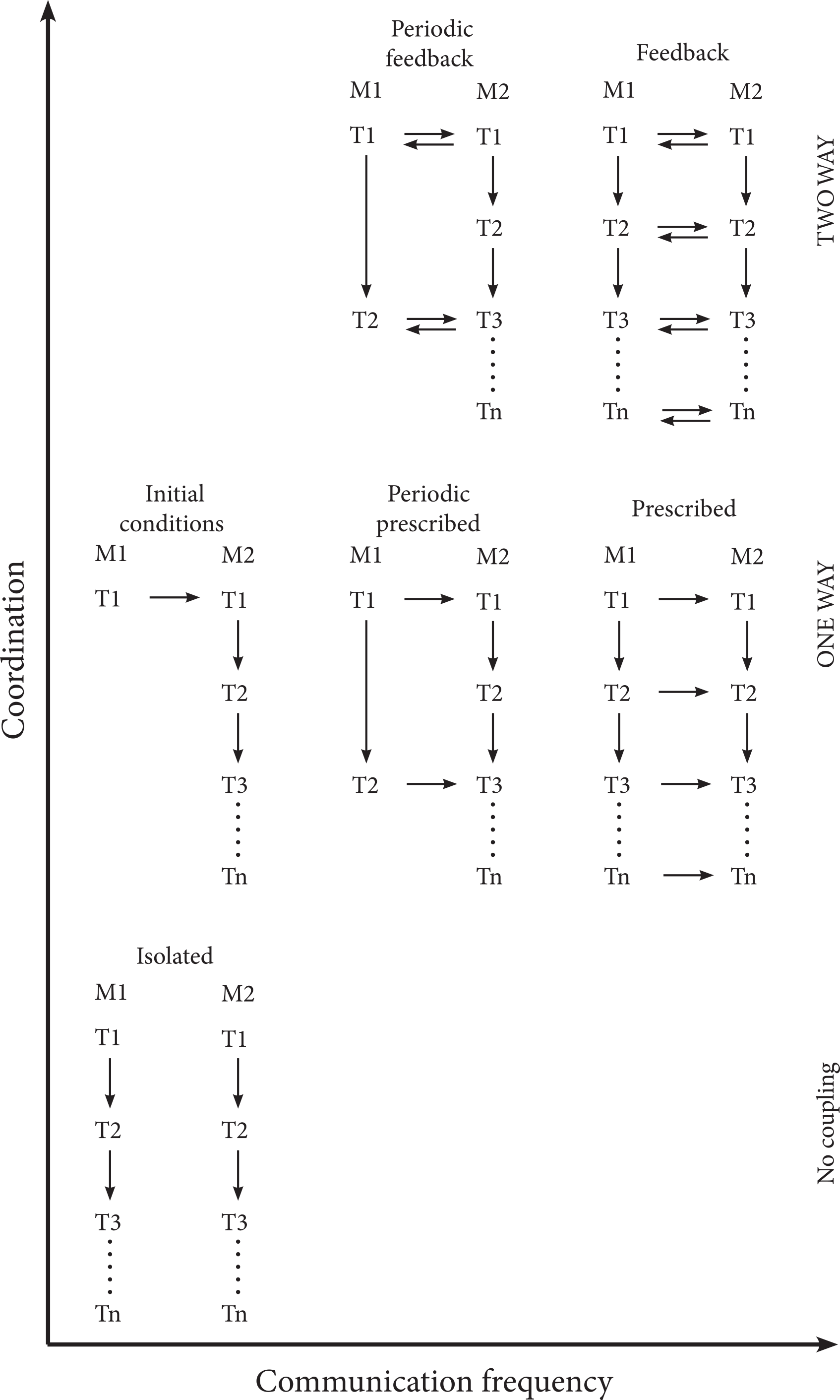
Figure 2Conceptual outline of the frequency of model communication and coordination of interaction between models from no coupling to one-way and two-way feedback. Examples are not exhaustive but illustrate common approaches used. M1: model 1; M2: model 2; T1: time step 1; Tn: time step n. Initial conditions, where one model is merely used to set the initial conditions of another; periodic perturbations, whereby one model updates data or variables used by another periodically and unilaterally; prescription, which is common to climate models that use a prescribed trajectory of land-cover data that do not endogenously change; periodic two-way feedback, whereby two different modelled processes may act at different temporal resolutions and feedbacks occur upon alignment; and two-way feedback where the modelled processes are dependent on the results and behaviour of each other.
Many existing instances of coupled models employ intermediate degrees of coupling. Existing technologies (i.e. couplers) that support model coupling deploy the strengths of tight and loose coupling approaches (Syvitski et al., 2013) in ways that address inherent trade-offs between control versus openness, high-performance computing versus wide distribution, distributed versus concentrated expertise, and shared versus modular independent code. In model coupling, couplers refer to independent software designed to manage the interaction between two or more models in terms of the passing of data, manipulation of parameters, and scheduling of processes between models and in some cases directing models to data or preprocessing data for use by a model. Typically, couplers are designed for independent research projects using known and available software (e.g. R) and programming languages (e.g. Java, C, Fortran). When a coupler has been designed for general use across multiple projects, the result is a coupling framework that enables the instantiation of multiple model coupling projects by others. Like existing modelling frameworks, a coupling framework can speed up the coupling process and facilitate the interaction, adoption, and comparison of different instantiated and coupled models.
Couplers or coupling frameworks (Fig. 1d–h) are typically introduced when a modelling project becomes multidisciplinary and requires collaborative modelling of several scientific disciplines, such that the coupled model is too complex to be comprehended by a single individual or research group (Voinov et al., 2010). For example, the Community Surface Dynamics Modeling System (CSDMS; Peckham et al., 2013) promotes distributed expertise and independent models in the domain of Earth-surface dynamics. All components are required to implement basic model interfaces (BMIs) as communication ports with any other components in CSDMS (Syvitski et al., 2014). Similarly, to enable interaction through a coupling framework (Fig. 1d), it has been suggested that all components implement the Earth System Modeling Framework (ESMF; Theurich et al., 2016), The Modular System for Shelves and Coasts (MOSSCO; Lemmen et al., 2018a) provides an example of this approach and combines the high-performance computing (HPC) capability of ESMF with the distributed expertise of CSDMS to facilitate access to HPC for those working to couple models without expertise with HPC.
The degree of coupling is important as a technical design question, as depicted in Fig. 1, but also as an important ontological question affecting how well we can represent feedbacks within and among human and environment systems (Ellis, 2015; Liu et al., 2015; Dorninger et al., 2017). Taken together, the frequency of communication and degree of coordination affect the degree to which feedbacks can be represented in coupled systems and, therefore, considered in our prediction of system behaviour or response to interventions (Fig. 2). For this reason, we describe four examples of coupled representations of human and natural systems, across a range of processes represented and scales of application, and how their coupling design affects the representation of feedbacks.
The four examples are situated at different points along the three dimensions of configuration, the frequency of communication, and coordination. The first example uses a coupler in its architecture (similar to Fig. 1d and f) and achieves two-way coupling (Fig. 2) to investigate the effects of land management on erosion. Our second example investigates the effects of land management on carbon storage using a loose coupling approach with two models, whereby one acts as a scheduler for the other (Fig. 1c) and both interact with common data to achieve two-way feedback (Fig. 2). The third example uses a coupler to bring together multiple models that share data (Fig. 1d) and create two-way feedback (Fig. 2) to investigate changes in land use and food consumption under climate perturbations. Our fourth and final example uses a coupler-based architecture (Fig. 1d) to tightly couple multiple models to investigate how changes in land use and the energy system affect terrestrial and atmospheric carbon storage and flux. While all four examples achieve two-way feedback (Fig. 2), most examples originated with one-way feedback (Fig. 2) or were constructed to enable an investigation of how the incorporation of feedback could alter model outputs. Collectively, the four examples illustrate how groups of researchers have attempted to overcome the lack of suitable frameworks for coupling human and natural systems and the lessons learned for future representations of feedbacks among human and natural systems.
2.1 Tight coupling – effects of subsistence agriculture and pastoralism on erosion
2.1.1 Model definition and description
The Mediterranean Landscape Dynamics (MedLanD) project developed a computational laboratory (Bankes et al., 2002) for high-resolution modelling of land-use–landscape interaction dynamics in Mediterranean landscapes called the MedLanD Modeling Laboratory (MML). MML is a virtual lab designed as a configurable and controlled experimental environment to couple representations of human and natural systems (Miller and Page, 2007; van der Leeuw, 2004; Verburg et al., 2016). The MML integrates an agent-based model (ABM) of households practicing subsistence agriculture and/or pastoralism and cellular automata models of vegetation growth, soil fertility dynamics, and landscape evolution (e.g. erosion/deposition) along with climate scenario data. The components of the MML are connected through a coupler that passes information between them (Fig. 3; Davis and Anderson, 2004, p. 200; Gholami et al., 2014; Sarjoughian et al., 2013, 2015; Sarjoughian, 2006) (see “Approaches to model coupling” section).
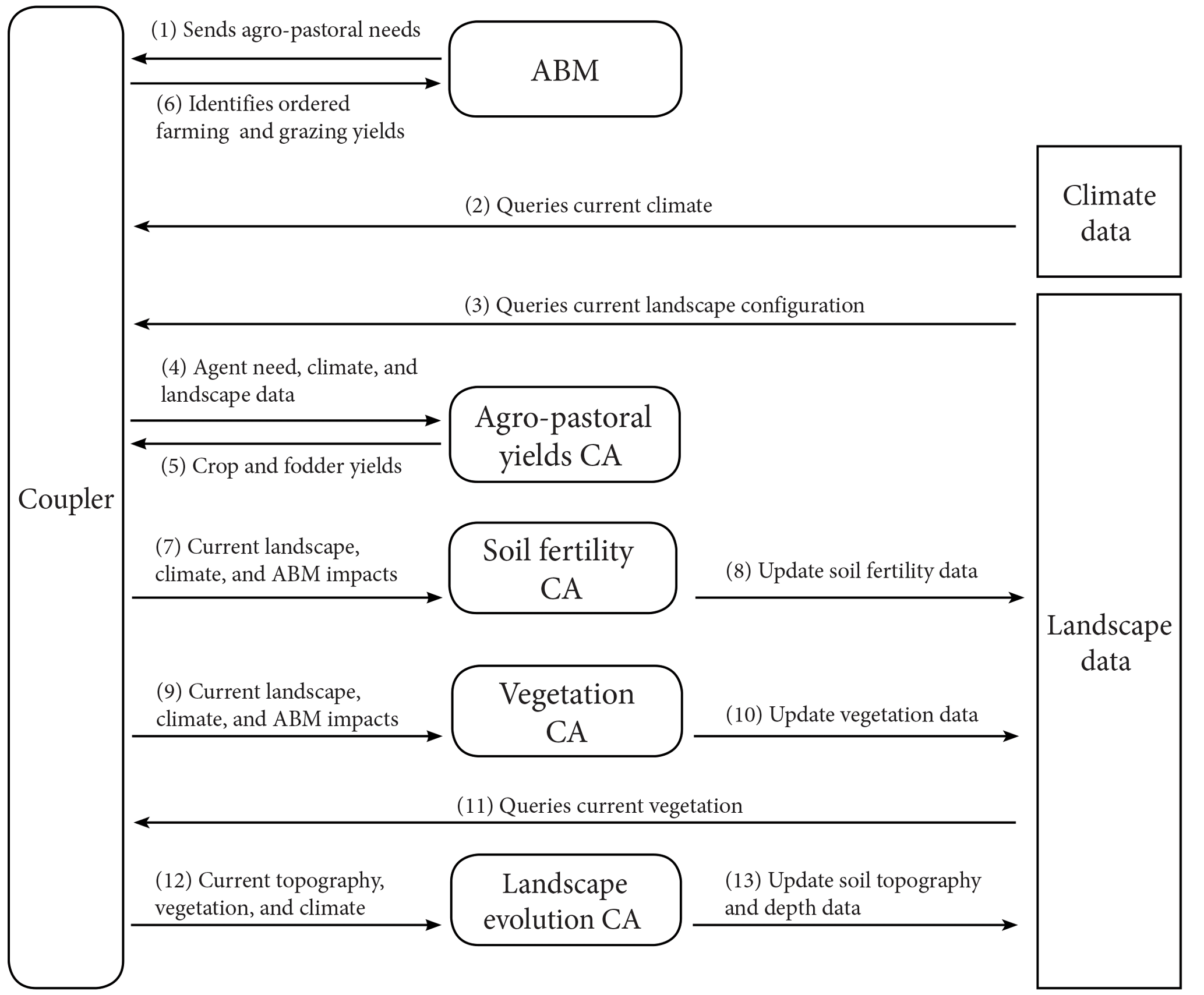
Figure 3Structure of feedback between the components of the MedLanD Modeling Laboratory, comprising an agent-based model (ABM), several cellular automata (CA) models, data, and a coupler. Numbers indicate the sequence of steps in a single time step of a coupled model run.
Villages and household actors are represented as agents in the ABM, which simulates land-use decisions and practices, mirroring the organization of known small-scale subsistence farmers (Banning, 2010; Flannery, 1993; Kohler and van der Leeuw, 2007). These agents select land for cultivation and grazing using decision algorithms and projected returns informed by studies of subsistence farming, with emphasis on the Mediterranean and xeric landscapes (Ullah, 2017).
The landscape evolution model (LEM) iteratively evolves digital terrain, soil, and vegetation on landscapes within a watershed by simulating sediment entrainment, transport, and deposition using a 3-D implementation of the Unit Stream Power Erosion/Deposition (USPED) equation and the Stream Power equation (Barton et al., 2016; Mitasova et al., 2013). The LEM also tracks changes in soil depth and fertility due to cultivation and fallowing. A simple vegetation model simulates clearance for cultivation or removal by grazing and regrowth tuned to a Mediterranean 50-year succession interval based on empirical studies in the region (Bonet, 2004; Bonet and Pausas, 2007). Climate parameters can be entered iteratively or statically and may derive from any external climate or paleoclimate data or simulation output.
2.1.2 Feedback implementation
The coupling architecture of the MML is highly structured, following a tight coupling scheme that is a hybrid of types shown in Fig. 1d and f. In the MML, a coupler manages much of the interaction with data, but it also coordinates the scheduling and exchange of data among the various subcomponent models. The coupler was constructed to query data directly and transform it for use by certain submodels but it also directs subcomponent models to run and independently retrieve data and produce output files. Coordination by the coupler is achieved through the use of a strict file naming system and the use of a common data format (e.g. spatial data must be in the GRASS geographical information system – GIS – raster file format (Neteler et al., 2012) and other data in delimited text files). Naming conventions of data files indicate data type, temporality, and data permanence (intermediary data versus final data). Two versions of the MML have been developed: one where the coupler is an independent piece of wrapping software coded in Java (in MML v1; Barton et al., 2015a) and one where the coupler is integrated into the main model codebase (in Python) of a reduced version of MML (in MML-Lite; Barton et al., 2015b). Subcomponent models are also either independent software scripts coded in Python (Landscape components) or in Java (ABM) in the MML v1 or are coded in a monolithic Python codebase in the MML-Lite.
The structure and sequence of a single time step of an MML simulation begins with the coupler initiating the ABM. The ABM determines the subsistence requirements for all households in the agent population and passes access to these data as a delimited text string back to the coupler (Fig. 3.1). The coupler then retrieves climate and landscape information and passes data file location information for subsistence requirements to the Agro-Pastoral Yields cellular automata (CA) submodel (Fig. 3.4). The Agro-Pastoral Yields CA submodel chooses locations for the various subsistence tasks and calculates yields that are returned in the form of a spatial data layer (i.e. a GRASS GIS raster file). Yields are then passed back to the ABM (Fig. 3.6) to determine the effects of subsistence choices for each household. At this time, the human system waits while several natural processes are simulated. The coupler calls the Soil Fertility CA to update soil characteristics degraded by land use (i.e. farming, grazing, or firewood gathering) and climate impacts. The coupler then calls the Vegetation CA to determine the amount of vegetation regrowth following agent land-use impacts (Fig. 3.9). Both the Soil Fertility and Vegetation CAs directly write output in the form of GRASS GIS raster files that are queried by the coupler at the beginning of each time step. Lastly, the coupler calls the landscape evolution model, which updates the land surface based on the new configuration of vegetation and climate data for that year.
The new state of the natural system (i.e. altered land surface, vegetation, and soils) affects household-agent decisions and natural-system processes (i.e. CA submodels) in subsequent time steps to achieve two-way feedbacks (as in Fig. 2, upper right). It is worth noting, however, that the MML currently only implements climate as a one-way prescribed coupling (Fig. 2).
2.2 Loose coupling – effects of residential land management on carbon storage
2.2.1 Model definition and description
To quantify the effects of residential land management on ecosystem carbon, a framework was developed to couple a human decision-making model with the dynamic global vegetation model BIOME-BGC (Robinson et al., 2013a). Our model of the human system, Dynamic Ecological Exurban Development (DEED) model, combines a suite of components developed to systematically incorporate additional data and complexity in the residential development landscape (Brown et al., 2004, 2008; Brown and Robinson, 2006; Robinson and Brown, 2009; Robinson et al., 2013a; Sun et al., 2014). Farmer agents own land that is bid on by residential developer agents. The winning residential developer agent subdivides the farmland into one of three residential subdivision types, each with different lot density and land-cover impacts (remove all vegetation, leave existing vegetation, grow new vegetation). Residential household agents then locate and conduct land management activities.
BIOME-BGC was used to represent deciduous broadleaf forest and turfgrass (i.e. maintained lawn) growth. It operates on a daily time step and reports outputs at daily and annual periods. Although the model was not developed to include land management, it was selected because (1) existing variables permit the representation of different types of vegetation found in exurban landscapes (Robinson, 2012) like turfgrass (Milesi et al., 2005); (2) the parameters and data used by the model can be altered to represent the impacts of land management that affect vegetation growth; (3) the biogeochemical cycling in the model represents water, carbon, and nitrogen with extensive literature validating model outcomes, including parameterization for different ecosystems and species (White et al., 2000); and (4) it has been applied both at high spatial resolutions (e.g. 30 m) and at local-to-global spatial extents (e.g. Coops and Waring, 2001), which facilitates both the local site evaluation and the potential to scale out to regional or national levels.
2.2.2 Feedback implementation
A loose coupling approach linking the ABM (DEED) and BIOME-BGC was used that is similar to the structure of Fig. 1c, whereby information is exchanged between data files. However, DEED not only modifies data files used by BIOME-BGC but it also coordinates its run time (Fig. 5). Through this approach, DEED is an independent model and a coupler coordinating interaction with BIOME-BGC.
By chaining the input and output between the two models, two-way feedback is represented (Fig. 2). First, land exchange, land-use change, and land management activities are conducted by agents in DEED. If agents irrigate their property then DEED modifies precipitation values in the climate files used by BIOME-BGC for that year and location. If agents fertilize, then DEED alters the soil mineral nitrogen in the BIOME-BGC initial conditions/restart file (Fig. 4.1). Then, DEED steps BIOME-BGC forward by 1 year (Fig. 4.2).
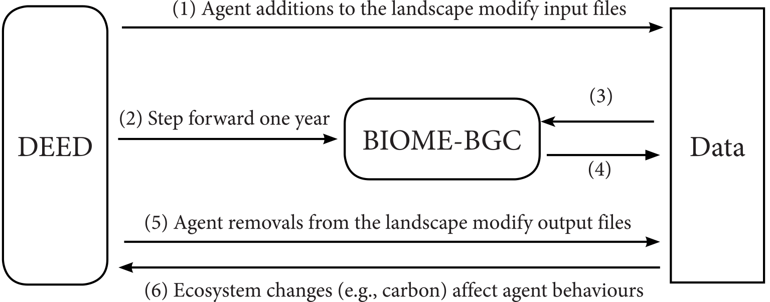
Figure 4Structure of feedback between DEED and BIOME-BGC. Numbers indicate the sequence of steps in a single time step of a coupled model run. (3) BIOME-BGC retrieves site-characteristic and climate data as well as initial conditions for the next time step comprising biogeochemical pool values among other information. (4) Results of vegetation growth and changes to biogeochemical pools are written back for manipulation by the ABM.
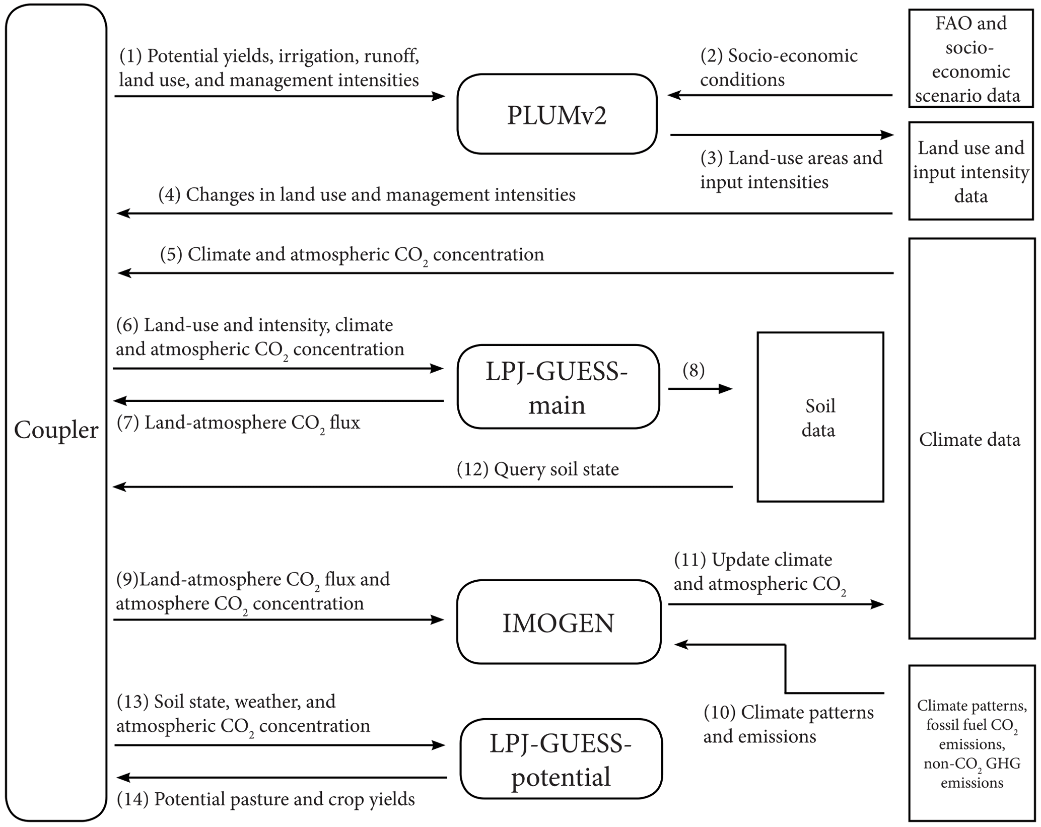
Figure 5LPJ-GUESS, IMOGEN, and PLUMv2 model coupling structure and feedback between models and data. Numbers indicate sequence of steps after initialization. (8) LPJ-GUESS-main modifies the soil state locational data.
BIOME-BGC retrieves site-characteristic, climate, and initial conditions for the year (Fig. 4.3). The products of vegetation growth from BIOME-BGC (i.e. coarse woody debris and litter) are then modified by land management activities by altering the initial conditions file for the subsequent year (Fig. 4.5). The ABM then summarizes ecosystem variables (e.g. carbon) for a given cell, residential property, or landscape. Feedback from the ecological system on agent behaviour was explored through changes in policies that support offset payments for increased carbon storage. An alternative feedback could include effects on social preferences and norms for landscape design elements (e.g. xeriscaping or adding tree cover) that may drive changes in land management activities and subsequent ecological outcomes.
2.3 Loose coupling with coupler – changes in food consumption and trade with land-use decisions
2.3.1 Model definition and description
To explore the interactions among land-use decisions, food consumption and trade, land-based emissions, and climate at a global scale, a dynamic global vegetation model (LPJ-GUESS; Smith et al., 2014), a land use and food system model (PLUMv2; Engström et al., 2016), and a climate emulator (IMOGEN; Huntingford et al., 2010) were coupled (Fig. 5). Key objectives were (a) to represent the trade-offs and responses between agricultural intensification and expansion and the cross-scale spatial interactions driving system dynamics (Rounsevell et al., 2014), (b) to explore whether climate and CO2-related yield changes in a coupled system would affect projected land-cover change, and (c) how these changes might feed back to the atmosphere and climate via the carbon cycle. A detailed representation of yield responses to inputs (fertilizers and irrigation) was used and assumptions of market equilibrium were relaxed to allow exploration of the effects of shocks and short-term dynamics.
The carbon, nitrogen, and water cycles, as well as vegetation growth, composition, and competition (e.g. following land-use change) were simulated at 0.5 ∘ spatial resolution in LPJ-GUESS. Agricultural and pastoral systems were represented as a prescribed fractional cover of area under human land use per grid cell. Four crop functional types modelled on winter wheat, spring wheat, rice, and maize were used to simulate croplands (Olin et al., 2015; Lindeskog et al., 2013; Pugh et al., 2015). Pastures were represented by competing C3 and C4 grass, with 50 % of the above-ground biomass removed annually to represent the effects of grazing (Lindeskog et al., 2013). A general circulation model emulator, IMOGEN, links the terrestrial and atmospheric carbon cycle without the computational demands of running a full Earth-system model (Huntingford et al., 2010).
Economic and behavioural aspects for country-level decisions within the food system were modelled in PLUMv2, extending Engström et al. (2016). The PLUMv2 model projects demand for agricultural commodities based on socio-economic scenarios (e.g. shared socio-economic pathways (SSPs); van Vuuren and Carter, 2014) and attempts to meet these demands through country level cost minimization, including spatially specific land-use selection among other processes such as trade and policy.
2.3.2 Feedback implementation
The coupling of IMOGEN, PLUMv2, and LPJ-GUESS is performed using a coupling script written in CRAN R (R Core Team, 2013), which coordinates data, settings files, and the order of operations for the three models similar to Fig. 1d. The coupling script first performs initialization steps, which produces the required start files and spins up all the models. As part of this process, IMOGEN is spun-up first (Fig. 5). IMOGEN provides spin-up climate for LPJ-GUESS and then PLUMv2. Two instantiations of LPJ-GUESS are used, one for simulated land-use conditions (LPJ-GUESS-main) and one for generating potential crop yields under a range of land uses (LPJ-GUESS-potential).
The coupling script communicates with the IMOGEN and LPJ-GUESS at a 1-year time step, although LPJ-GUESS and IMOGEN operate on sub-daily time steps. IMOGEN is called to provide the climate for the current run year (Fig. 5.9, .11), which LPJ-GUESS-main uses (Fig. 5.5) to simulate the vegetation dynamics with the climate from IMOGEN and the land use from PLUMv2 for the same year (Fig. 5.3, .4, .6)). The terrestrial carbon flux data are aggregated to provide global net ecosystem exchange of carbon for the land area with prescribed ocean carbon uptake to IMOGEN, which estimates the global CO2 concentration and climate for the next year.
Every fifth year, the R coupler runs a second instantiation of LPJ-GUESS (LPJ-GUESS-potential), directing it to use the ecosystem soil state of LPJ-GUESS-main (Fig. 5.12, .13). The LPJ-GUESS-potential model is used to produce potential net primary production (NPP) for pasture grasslands and potential crop yields for six crop management settings (three levels of fertilization (0, 200, 1000 kg N ha−1) and rain fed or irrigated crops). To account for short-term land-use change legacy effects, LPJ-GUESS-potential uses the previous 10 years of soil conditions and climate from IMOGEN. The last 5 years of the LPJ-GUESS-potential pasture NPP and crop yields are averaged by the R coupler and input to PLUMv2 (Fig. 5.1) to model land use for the next 5-year iteration. PLUMv2 uses these yield potentials to simulate annual land-use management decisions, which are used (as described above) in the LPJ-GUESS-main model (Fig. 5.4, .6). The land uses are determined using yield potentials for previous time periods in LPJ-GUESS-potential and therefore has been indicated as step 1 in Fig. 5.
2.4 Tight coupling via a coupler – investigating the effects of changes in land use and the energy system on terrestrial and climate CO2
2.4.1 Model definition and description
The integrated Earth System Model (iESM v1.0; Collins et al., 2015a) couples the Global Change Assessment Model (GCAM, v3.0; Wise et al., 2014) with the Community Earth System Model (CESM, v1.1.2; Hurrel et al., 2013) and the Global Land-use Model (GLM, v2; Hurtt et al., 2011) to explore feedbacks between terrestrial ecosystems (including their interactions with the climate system) and human land use and energy systems. GCAM is an integrated assessment model that represents both human and biogeophysical systems (Wise et al., 2014), and in the iESM the climate and carbon components of GCAM are replaced by CESM. The human components simulate global energy and agriculture markets to estimate anthropogenic emissions and land change. The energy and land components are distinct but connected via bioenergy, nitrogen fertilizer, and (where applicable) greenhouse gas emissions markets. GLM generates annual, gridded land use from periodic, regional GCAM outputs following the Land Use Harmonization protocol (LUH; Hurtt et al., 2011), and an additional land-use translator converts GLM outputs to CESM land-cover types (Di Vittorio et al., 2014; Lawrence et al., 2012).
CESM is a fully coupled Earth-system model with atmosphere, ocean, land, and sea ice components, including land and ocean biogeochemistry that exchanges carbon with the atmosphere (Hurrel et al., 2013). The standard resolution of all CESM components in fully coupled mode is nominally 1 ∘, but the land cover is determined as fractions of half-degree grid cells and prescribed prior to a simulation (Lawrence et al., 2012). Biogeographical vegetation shifts are not included, although ecosystems do respond and contribute to changing environmental conditions. The CESM land model includes detailed hydrology and mechanistic vegetation growth for 16 plant functional types (PFTs) to simulate water, carbon, and energy exchange with the atmosphere.
The iESM coupling follows the Coupled Model Intercomparison Project phase 5 (CMIP5; Taylor et al., 2012) LUH protocol (Hurtt et al., 2011), with some modifications and additions (Bond-Lamberty et al., 2014; Di Vittorio et al., 2014), to connect GCAM and GLM (Hurtt et al., 2011) directly to the CESM framework via a newly developed integrated assessment coupler (Collins et al., 2015a).

Figure 6Structure of iESM and feedback between integrated model components. An integrated assessment coupler facilitates all interactions between the Global Change Assessment Model (GCAM), the Global Land-Use Model (GLM), and the Community Earth System Model (CESM). The coupler is activated by the CESM land model every 5 years to calculate the average carbon and productivity scalars for the past 5 years and pass them to GCAM, then pass GCAM outputs to the atmosphere component of CESM via a downscaling algorithm and to GLM, and then pass GLM outputs to the land component via a land-use translator (LUT). The non-CO2 emissions are provided to CESM as an input data file.
2.4.2 Feedback implementation
The outputs generated by the two-way feedback (Fig. 2) between the human and natural systems represented by iESM are not available from its individual models or through one-way coupling such as in CMIP5. The iESM is a specific configuration of CESM in which the land model initiates an integrated assessment coupler every 5 years (Fig. 6.1). This coupler coordinates communication between the human and environmental systems by first calculating average crop productivity and ecosystem carbon density scalars from the previous 5 years of CESM net primary productivity and heterotrophic respiration outputs (Bond-Lamberty et al., 2014), except during the initial year when these scalars are set to unity (Fig. 6.2). The coupler then runs GCAM with these scalars to project fossil fuel CO2 emissions and land-use change for the next 5 years (Fig. 6.3), and then passes these outputs through downscaling algorithms to the atmosphere and land components of CESM (Fig. 6.4–.9). The non-CO2 emissions are prescribed by CMIP5 data as initial CESM input files. Land-use change is annualized and downscaled by GLM (Hurtt et al., 2011) (Fig. 6.4, .5). A land-use translator converts these changes in cropland, pasture, and wood-harvested area into changes in CESM land-cover change, which is based on plant functional types (Di Vittorio et al., 2014, Lawrence et al., 2012) (Fig. 6.6, .7). The CO2 emissions are downscaled following Lawrence et al. (2011) and passed to the atmosphere component as a data file (Fig. 6.8), and the land-cover change is stored in a land surface file and passed to the land component (Fig. 6.9). The coupler then returns control to the land model and CESM runs for another 5 years (Fig. 6.10). This two-way feedback incorporates the effects of climate change, CO2 fertilization, and nitrogen deposition on terrestrial ecosystems into GCAM's projections.
The key new feature is the generation of CESM-derived vegetation and soil impact scalars that are used by GCAM to adjust crop productivity and carbon at each time step. This fundamentally alters the scenario by making the land projection, and consequently the energy projection, more consistent with the climate projection. The largest technical contribution, however, is the integrated assessment coupler that enables feedbacks by running GCAM, GLM, and a new land-use translator inline with CESM.
These capabilities enable new insights into research questions regarding climate mitigation and adaptation strategies. For example, how may agricultural production shift due to climate change, how do different policies influence this shift, and how may this shift affect other aspects of the human–Earth system? Many recent impact studies (e.g. ISIMIP, BRACE, CIRA2.0) use climate model simulations based on emissions and land-use scenarios (Representative Concentration Pathways, RCPs) that themselves do not account for the influence of climate change on future land use. This inconsistency could affect conclusions about impacts resulting from particular RCPs.
This approach paradoxically has several strengths that are also weaknesses. The main strength of this approach is that it tightly couples two state-of-the-art global models to implement primary feedbacks between human and environmental systems under global change. Unfortunately, this configuration is not amenable to the uncertainty and policy analyses or the climate target experiments usually employed by GCAM because it takes too long to run a simulation. As a global model it provides a self-consistent representation of interconnected regional and global processes, both human and environmental, but is unable to capture a fair amount of regional and local detail that influences planning and implementation of adaptation and mitigation strategies.
The four presented examples demonstrate how specialized models of human and natural processes have been connected through alternative coupling approaches to address research questions related to the impacts of one system on another and the effects of feedbacks between human and natural systems on a variety of outcomes of interest (e.g. erosion, carbon storage, and emissions). The focus on specialized models offers a flexible and open approach to answering new questions about feedbacks in coupled human–natural systems and also facilitates the identification of new types of data required to calibrate and validate the interactions and feedbacks between the two systems. Additionally, coupled modelling presents an opportunity for increased transparency and detail in the represented processes through more explicit identification and documentation of component interactions and processes.
The example models are diverse in the spatial and thematic resolutions of human- and natural-system processes represented. The first two examples (MML and DEED) use agent-based approaches that represent land use and land management in the human system at the household level. While the ecological impact of land management activities in DEED does not have a direct feedback on residential household decision making, those represented in MML do. Agricultural systems, carbon markets, and policies provide mechanisms to establish this feedback and endogenize the impact-response cycle between residential land management practices of the human system and the natural system (Sun et al., 2014).
The second two examples are global models with different levels of coupling and complexity that represent human–natural-system feedbacks at regional and global levels. In both examples, the human system has a direct effect on modelled natural-system processes (i.e. vegetation, carbon, climate), and the feedback of environmental changes on human systems is mediated by vegetation responses to changing natural and human conditions.
These examples demonstrate how coupled system implementations extend the applicability of models to a variety of questions regarding the dynamic relationship between human and environmental systems that would otherwise be impossible to address quantitatively. Such questions include those related to direct and indirect effects of one system on another (e.g. what is the effect of the natural system on the human system?), to the resilience or sensitivity of the coupled system or its components to perturbations or scenarios (e.g. do feedbacks dampen or amplify the consequences of a perturbation?), and to identifying thresholds (e.g. what is the critical value of a variable in one system that when crossed instantiates change in the other system?), among many others.
3.1 Lessons learned
To make progress in modelling coupled human–natural systems, the way in which some set of variables or processes affects or interacts with both systems must be specified. For example, precipitation has a known and direct effect on plant growth (e.g. forest or crop) and erosion (e.g. overland flow). The outcomes of some of these processes (e.g. yield and soil loss) have direct or indirect effects on land management choices by farmers, effects that are empirically observable at least qualitatively and, in some instances, quantitatively measured. However, the direct impacts of other perturbations, such as the introduction of new technology or governance schemes, on human- and natural-system processes are not observable because they have not yet occurred. The presented case studies focus on perturbations or scenarios that are grounded in known and direct causal relationships that are more likely to be found in the natural system than the human system, partly due to the multitude of drivers affecting—and consequent difficulty in predicting—human-decision making. In these example cases, a number of lessons have been learned:
-
Lesson 1: leverage the power of sensitivity analysis with models. A powerful benefit of simulation models is that they can facilitate analysis of the effects of interventions and scenarios for which there is no precedent. Models should be leveraged through computation across a full range of parameters and use of simulated data or expert- or theory-informed methods to evaluate the relative contribution of parameter values/ranges, missing data, or processes on model outcomes. For example, to properly understand the net effect of human alteration to vegetation on long-term rates of erosion and deposition in the MML, it became clear that a more complete understanding of the sensitivity of the landscape evolution subcomponent model to vegetation was needed. This sensitivity analysis showed a very strong exponential relationship between vegetation type and both the overall amount of erosion and deposition over time and the temporal variation in erosion rates over time (Ullah, 2017), The analysis show a particular sensitivity to expanded bare land, grasslands, and shrub land-cover types. Therefore, it is clear that agent activity that leads to an increase these types of land cover should also lead to long-term increases in erosion and deposition in the MML. In this way, model sensitivity to parameters, data, or processes can be evaluated to support design and deployment of resources for new data collection.
-
Lesson 2: modelling is an iterative process. The process of analyzing coupled human- and natural-system models often results in the identification of needs to investigate key variables, data, or mechanisms. For example, through the coupling of DEED and BIOME-BGC (Sect. 2.2), it was realized that data on vegetation and soil carbon for residential land uses are grossly inadequate for model calibration. This realization fostered new data collection and analysis about the distribution of carbon stored in different residential land uses (Currie et al., 2016). New forms of measurement and evaluation are often needed to collect novel data and quantify variables and feedbacks linking human and natural systems. As these new data are collected and become available, new questions about model processes are inevitable (Rounsevell et al., 2012).
-
Lesson 3: create a common language. Coupling human and natural systems brings social and natural scientists together that often have a different understanding of the meanings of commonly used terms. Both technical and conceptual aspects of the coupling process can be improved when a common language is used. For example, traditional coupling between the ocean and the atmosphere in Earth-system models typically uses the climate and forecast conventions (Eaton et al., 2011). A controlled vocabulary in these conventions assists the understanding of model processes and facilitates their coupling among models or replacement in new models. With a similar goal but different approach, CSDMS introduced rules for the creation of unequivocal terms through their standard names system that function as a semantic matching mechanism for determining whether two terms refer to the same quantity with associated predefined units. This concept is currently undergoing transition to a geoscience standard names ontology that reaches out to include social science terms (David et al., 2016), which can benefit communication between communities (i.e. natural and social science) that may have different terms and descriptions of similar processes (Di Vittorio et al., 2014). With a common language, data can be more easily and unambiguously communicated between components in a coupled system.
-
Lesson 4: make code open-access. Many ecosystem and Earth-system models have mass, energy, or other balance equations that constrain the processes to the laws of thermodynamics and can be used to ensure that they are working correctly. For example, the ecosystem model LPJ-GUESS has a routine to ensure balance between influx, efflux, and storage of carbon. Similar checks and balances are used in human-system models with respect to population change (e.g. births, deaths, immigration, and emigration) or economic trade (e.g. production, consumption, imports, and exports) at macro levels and budget or labour constraints at household or individual levels. However, in many natural-system models these balance equations are not accessible for coupling and the representation of human perturbations and modifications to the factors in balance equations are either not included or done so indirectly and make the coupling less flexible and tractable. Moving forward, critical equations, like mass balance equations, and model variables should be made open through coding to provide multiple points for interfacing with other models (specifically human-systems models).
-
Lesson 5: ensure consistency. Modelers seeking to couple natural- and human-systems models that represent similar phenomena, like land cover, can encounter significant ontological and process consistency challenges. Models with different initial assumptions and different processes can generate different values for the same phenomenon. While model coupling can ultimately provide an impetus for harmonizing and resolving such consistency issues, it requires decisions about which processes to represent and which to leave out to avoid duplication.
The iESM (Sect. 2.4) illustrates issues of consistency in assumptions, definitions, and processes well. First, ecosystem properties from CESM were translated to impacts that could be applied to GCAM “equilibrium” yields and carbon densities (Bond-Lamberty et al., 2014). Second, a major finding that is especially relevant to all land change and ecosystem models is that the inconsistencies between land use and a land-cover definition caused CESM to include only 22 % of the prescribed RCP4.5 afforestation in CMIP5 (Di Vittorio et al., 2014). Additionally, it was discovered that wood harvest was conceptually different across the three models comprising iESM (GCAM, GLM, and CESM), with each model having its own process for determining how harvest is spatially distributed. Wood harvest is a good example of different modelling groups describing the same thing and using the same language but with very different concepts and processes, with unintended consequences for CESM's terrestrial carbon cycle.
-
Lesson 6: reconcile spatio-temporal mismatch. Many natural-system models operate at finer temporal and coarser spatial resolutions than human-system models (Evans et al., 2013). Often, these discrepancies cannot simply be dealt with by aggregation of the variables because they represent mismatch in spatial and temporal dynamics that may also happen in reality. Human responses to environmental change may show significant time lags or may be related to cycles of management (e.g. cropping cycles) rather than showing an immediate response. Similarly, while the ecological models are strongly place-based, coupling human and natural systems at the pixel level may not always be appropriate due to complex spatial relations in the human dimensions (e.g. distant land owners) or responses across different levels of decision making (e.g. policy responses) that are not linked to the exact place of the ecological impact. Reconciling these mismatches involves balancing detail and computational tractability within existing model structures and scheduling the frequency of communication between models.
As an example, the DEED ABM (Sect. 2.2) used an annual time step to reflect the timing of land management decisions, whereas the ecosystem model BIOME-BGC represented vegetation growth and biogeochemical cycles daily. To reconcile these differences, irrigation decisions were made annually but implemented 1 day a week during the growing season by modifying the daily precipitation file used by BIOME-BGC. In contrast, other management activities were implemented once annually before (for fertilization) and after (for removals) the growing season. These limitations could have a significant effect on estimated carbon storage and have fostered additional fieldwork for further validation (e.g. Currie et al., 2016) and additional efforts to tightly couple the two models.
The iESM (Sect. 2.4) also reconciles similar mismatches through a 5-year time lag and specialized spatial and temporal downscaling of economic model outputs to provide inputs to the environmental model. While these approaches allow the separate models to operate synchronously, further development to better match the inherent spatio-temporal configurations between models is required to reduce errors associated with such mismatches.
-
Lesson 7: construct homogeneous units. Coupling models increases computational overhead and thus requires increases in computational efficiency, both of which come with trade-offs. One approach to improving efficiency is to classify and generalize components of the model such as agent types in the human system (e.g. Brown and Robinson, 2006), types of vegetation (e.g. plant functional types, Díaz and Cabido, 1997; Smith et al., 1993, 1997), or landscape units. Landscape units are not typically constructed to structure spatial variability in land-use science, but are used regularly in hydrological modelling; for example, the Soil Water Assessment Tool (SWAT; Neitsch et al., 2011) uses hydrological response units (HRUs) that have a soil profile, bedrock, and topographic characteristics that are assumed to be homogeneous for the entire spatial extent of the unit. Similar concepts have been used to identify management zones or units, and our examples of DEED-BIOME-BGC (Robinson et al., 2013a) and the iESM (Collins et al., 2015a) both employed this approach. However, the variability among management activities and land-cover types can lead to a large combination of outcomes, and the delineation of these units directly contributes to uncertainty in model projections (Di Vittorio et al., 2016).
-
Lesson 8: incorporating feedback increases non-linearity and variability. Specific results from the four examples are available in a number of publications associated with each example. Among the four example coupling efforts, it has been found that the incorporation of two-way feedbacks (Fig. 2) between models of the human and natural system typically produces non-linear results and a greater range in model outcomes than are observed when the models are isolated or one-way prescriptions are used. For both the MML and DEED models, changes in the natural system were relatively linear when one-way human perturbations were prescribed. However, when feedbacks between the systems were incorporated then non-linear outcomes and frequently a greater variation in model outcomes were observed.
3.2 Feedback effects
Introducing feedbacks often changes model outcomes, but it is difficult to determine if these changes are significant or realistic relative to the uncertainty in the original models and their coupling. The only way to test if the representation of a mechanism is representative of the real world is to remove the inconsistencies so that the feedback effects can be quantified. Then, experiments that evaluate the effects of specific feedbacks can be carried out and evaluated. These experiments need to be carefully designed because the actual feedback signal can be an aggregate of expected, direct effects and additional, indirect effects. For example, average ecosystem productivity could change due to atmospheric influences (e.g. climate change, CO2 fertilization) or to terrestrial influences associated with changing ecosystem area (e.g. spatially heterogeneous soil properties, changes in the proportion of different forest types). Regardless of the challenges, an overall benefit of quantifying feedback effects is that modellers can gain insight into processes that are typically not observed and measured. Given the difficulty in observing these effects and potential inconsistencies, efforts in coupling human- and natural-system models have focused on sensitivity analysis to test their effects (e.g. Harrison et al., 2016).
Ultimately, an important goal in such analyses is to discern which of two distinct sources produce effects from including feedbacks in coupled models: (1) model implementation (both technical and conceptual) and (2) the actual feedback signal. Model implementation issues often relate to the level of consistency between the original models. For example, the need to translate changes in gridded patterns of ecosystem productivity to changes in regional average carbon density can lead to varying sensitivities across magnitudes of productivity and areal change, requiring the unrealistic sensitivities to be filtered out (Bond-Lamberty et al., 2014).
Model experiments are useful for separating the model implementation issues from the actual feedback signal. For example, iESM was used in a series of land-only simulations to (a) quantify the relationship between ecosystem productivity and carbon density, (b) implement a statistical method to remove outliers that introduce error due to extreme combinations of land cover and productivity change, and (c) develop the appropriate proxy variables for use by GCAM (Bond-Lamberty et al., 2014). To verify that this process effectively removed the model implementation effects, another series of land-only simulations was conducted using the iESM with and without terrestrial feedbacks and with constant atmospheric conditions (i.e. year 1850 aerosols and nitrogen deposition, and repeating 15 years of climate forcing). This experiment showed that the coupling itself, without an atmospherically driven feedback signal, did not generate significant changes in GCAM outputs. The feedback signal was not zero, however, indicating that a combination of implementation effects and land heterogeneity effects was present. These combined effects were not separable due to lack of data on the required outputs, and in general they were opposite to the total feedback effects in the fully coupled iESM experiment, suggesting that the atmospherically driven feedbacks may be larger than the net feedbacks.
Depending on the mechanisms involved, feedbacks may create strong feed-forward effects that lead to a fast evolution of the dynamics of the system. By contrast, responses may also lead to an attenuation of perturbations and strong stability of the dynamics. Where the exact mechanisms involved and the strength of the feedbacks are unknown, model dynamics may start deviating strongly upon small changes in variable settings, in other words, leading to strong model sensitivity to highly uncertain model parameters.
The examples including feedbacks in coupled human–natural-system models illustrate a number of challenges in designing and implementing feedback mechanisms:
-
The representation of human responses. The examples in the four cases above mostly relate to a coupling based on exchanging land-cover and ecological-process-impact information. The human decision models translate the ecological impacts to alter decision making. For example, land-use decisions in PLUM-LPJGUESS, iESM, and MedLanD respond to changes in potential yields; in the MedLanD application, erosion processes also render land less suitable for use. In reality the responses of human decision making are more complex. The relevance of the ecological indicator exchanged may be context dependent; e.g. potential yields may determine farming decisions in capital intensive farming that is near to the production frontier but may be much less important in low-input subsistence farming that is far from potential productivity. Furthermore, decision making may not be based on the represented process or the indicator exchanged but rather on the human perception of the environmental change, which may be irrational and biased by other interests, such as in the case of the climate debate. While the concept of environmental cognitions is well known, relatively little is known in relation to land-use change decision making (Meyfroidt, 2013a). Human responses to environmental change are, therefore, a critical knowledge gap for implementing coupling mechanisms (Meyfroidt, 2013b).
-
Structural differences in model concepts. The iESM example illustrates how structural differences in models can hamper the coupling of models, and how careful consideration is needed of the feedback mechanism and its consequences in relation to the overall model assumptions. This is especially relevant for coupling models that assume equilibrium and those that depict instantaneous impacts or transient situations. Global economic models using equilibrium assumptions, which are frequently coupled to land-use and ecosystem models and specialized land-change models (or land-change modules in IAM models) both address land use but often from different perspectives leading to potential differences in the meaning and interpretation of input and output variables.
-
Reconciling stochastic and deterministic approaches. Another factor complicating the representation of feedback mechanisms is that some models are strongly deterministic (e.g. PLUM-LPJGUESS, GCAM-CESM – iESM, BIOME-BGC), so that the results are essentially the same for any run with the same initial parameters, while others have strong stochastic components (e.g. DEED and MedLanD). The former is common for many natural-systems models and some human-systems models (especially econometric style models). Other models have algorithms that generate stochasticity to represent uncertainty in processes. Many agent-based/individual-based models and some cellular automata fall into this category. For models with included stochasticity, the same random number generator seed can be used; however, to capture the variance and distribution of model outcomes, repeated runs with different seeds are required, which can be conceptually challenging or operationally complicated when coupled with deterministic models.
3.3 A way forward
The ability to dynamically simulate feedbacks between human decision making and natural processes requires some kind of tight coupling – in the sense of frequent, two-way communication and high coordination (Fig. 2) – between models designed to represent these different processes. To date, this has largely been achieved through connecting models into a single modelling environment. This is true to a large extent for all the case studies presented here. Adding new models to such systems often requires significant reprogramming and makes the expanded code base increasingly difficult to debug, verify, and validate. Additionally, any other researcher that would like to combine fewer, more, or different components will need to reprogram multiple parts of the modelling environment to decouple one model and add another.
To expedite coupling in future modelling of the land system, we recommend a bottom–up approach to modelling whereby modelers with in-depth domain knowledge create relatively small, more easily verified modules (Bell et al., 2015) or model components for assembly into larger coupling frameworks (e.g. OpenMI, ESMF, OMS, and CSDMS). Using this approach, the community may preserve and build upon existing numerical code previously developed by the many subdisciplines involved in modelling human and natural systems. These are not new ideas, but they have not yet been achievable in spite of their recognized desirability. However, a suite of technologies has reached sufficient maturity that it may now be a practical way to create a new generation of modelling tools that can exploit these two avenues for modelling coupled human–natural systems.
New coordinating frameworks for next generation coupled modelling of human and Earth systems are being developed within a number of relevant organizations: the CSDMS, the Network for Computational Modeling in Social and Ecological Sciences (CoMSES Net), and the Analysis, Integration, and Modeling of the Earth System (AIMES) Core Project of Future Earth. These frameworks envision a set of community-developed and endorsed standards for open, platform-independent model coupling and integration based around an interrelated set of components that build on lessons 3–6.
-
Start with wrapper container software (e.g. Docker) to encapsulate model code and dependencies needed.
-
Use a standardized API, like the extension of the Basic Modeling Interface (BMI) developed by the CSDMS, to standardize and describe various functions (e.g. model control, model information, time, variable information, variable getters and setters, and model grids) such that a calling component in the framework is provided with the level of control needed to access other component's metadata and simulated data (Hutton et al., 2014).
-
Incorporate Standard Names to map variables of multiple components to each other. In the CSDMS framework the Standard Names functions as a semantic matching mechanism, a lingua franca, for determining whether two variable names refer to the same quantity with associated predefined units.
-
Mitigate sunk-cost effects for integration into any one coupling framework by creating separate interfaces to one or more coupling frameworks (Peckham et al., 2013; Lemmen et al., 2018a).
-
Adopt reproducible workflow environments to wire models together, supervise their execution and manage the storage of the intermediate and final results needed for subsequent analysis.
For these elements of a framework to be maintained, a community organization is required in an open-source development environment. Models meeting these community standards would then be certified in public code libraries like those maintained by CoMSES Net and CSDMS to indicate which models could be coupled with any other certified model. Certification from a community organization and buy-in from the modelling community would create an ecosystem of open, connectable models that could be integrated into reproducible computational pipelines in standard ways for coupled human- and natural-system models. The evolution of such an ecosystem is dependent on the commitment of organizations representing modelling science to support and maintain a set of community standards and to facilitate the education and adoption of those standards by the modelling community. An important advantage of the proposed framework is that it does not require scientists to significantly change the way they develop models or to commit to a particular language, platform, or operating system. The combination of this development flexibility with committed standards and adoption assistance would enhance the likelihood of reaching a critical mass of development that would greatly expedite not only the development of coupled human- and natural-system models, but also increase the rate of scientific discovery in this domain.
Coupling human-system and natural-system models requires connecting distinct research fields, each with unique knowledge, methods, assumptions, definitions, and language. Success depends on the research team members learning enough about the other field and model to unambiguously communicate with each other, recognize strengths and weaknesses of other methods, translate assumptions and definitions, and critically evaluate other model processes and outputs. Additionally, some team members need to develop working expertise of both models and fields to facilitate the implementation of an internally-consistent coupled model. Furthermore, a software engineer is often needed to address the technical challenges of coupling complex models. Ultimately, the social and conceptual challenges combine to require much more time and effort for successful completion than for similar, mono-disciplinary projects. Nonetheless, all authors noted that the greatest benefit of the coupling process was the collaborative learning process that created a group of people with a working knowledge of both human- and natural-system research and expertise in how to integrate the two.
While successful coupling of human- and natural-systems models requires truly interdisciplinary collaboration, we note that the playing field is not level with respect to disciplines. There are more resources and active modelling efforts in the natural sciences than in human-systems science. This is unfortunate since natural scientists need to closely work with human-systems scientists to understand the kinds of information needed and the kinds of information that can be provided by models of human systems. Moreover, the most scientifically and socially valuable results of model coupling require that both natural-systems models and human-systems models be modified and enhanced to work together. The collaborative model development that this entails involves social interactions, two-way communication, and mutual respect for domain knowledge as well as technical solutions. In this regard, there needs to be scientific, professional, and policy incentives for all members of the interdisciplinary teams needed to develop successful integrated modelling.
These efforts highlight the difficulty and challenges associated with the process of human–environment model coupling as well as the opportunities that coupling presents for making substantive and methodological advances in science associated with human systems, natural systems, and their feedbacks on each other.
The underlying models and frameworks discussed in the presented research can be found through the URLs and DOIs provided below. The range of documentation and support for each model or framework varies. It should be assumed upon downloading that no support is available. While the posting of these models promotes transparency, their creation has involved teams of individuals who hold extensive experience and tacit knowledge working with the models and frameworks. The authors caution against their use and evaluation for scientific results without collaboration or consultation with their developers or members of their research teams.
The MedLanD Modeling laboratory can be referenced as Barton et al. (2018). The DEED conceptual model can be cited as Robinson et al. (2013a) with code retrieved from Robinson et al. (2013b). The PLUMv2 conceptual model can be cited as Alexander et al. (2018) with code retrieved from Alexander and Henry (2018). The LPJ-Guess conceptual model can be cited as Smith et al. (2014) and code requested from the authors. The iESM conceptual model can be cited as Collins et al. (2015b), with Version 1 code retrieved from Collins et al. (2015b). The CSDMS standards (CSDMS Integration Facility, 2018a), framework (CSDMS Integration Facility, 2018b), and software and model repositories (CSDMS community contribution) are made available on github. The MOSSCO model coupling framework can be retrieved from Lemmen et al. (2018b).
The authors declare that they have no conflict of interest.
This article is part of the special issue “Social dynamics and planetary boundaries in Earth system modelling”. It is not associated with a conference.
This research has been made possible for the authors from a variety of
supporting institutions, which we thank and acknowledge in what follows.
Derek T. Robinson was supported by the Natural Sciences and Engineering Council (NSERC) of
Canada as part of their Discovery Grant program. Alan Di Vittorio was supported by the
US Department of Energy, Office of Science, Office of Biological and
Environmental Research, Climate and Environmental Sciences Division,
Integrated Assessment Program, under Award Number DE-AC02-05CH11231. Peter Alexander,
Thomas A. M. Pugh, and Mark Rounsevell were supported by the Future Earth AIMES project, CSDMS, and the
European Commission LUC4C project. Almut Arneth, Sam S. Rabin, and Mark Rounsevell also acknowledge LUC4C
(grant no. 603542) and the Helmholtz association through its ATMO programme
and its Integration and Networking fund. Thomas A. M. Pugh was supported by the
University of Birmingham, the Birmingham Institute of Forest Research (BIFoR paper no. 30). C. Michael Barton and Isaac Ullah were supported by the
US National Science Foundation (grants BCS-410269, DEB-1313727, and GEO-909394),
and the support from Arizona State University and the Universitat
de Valencia, Spain. Many other people in Jordan, Spain, and the US
contributed in various ways to the MedLanD project, and we want to extend our
thanks to them also. Albert Kettner and James P. Syvitski were supported by the CSDMS project, funded
by The US National Science Foundation (grant 0621695). Carsten Lemmen was supported by
the MOSSCO project funded by the German Ministry of Education and Science (BMBF)
under grant agreements 03F0667A. Brian C. O'Neill's contribution was based upon work
supported by the National Science Foundation under grant number AGS-1243095.
Peter H. Verburg was supported by the European Union's Seventh Framework Programme ERC grant
agreement no. 311819 – GLOLAND.
Edited by: Jonathan Donges
Reviewed by: three anonymous referees
Alexander, P. and Henry, R.: PLUMv2, https://bitbucket.org/alexanpe/plumv2/src/RCP paper, last access: 18 June 2018.
Alexander, P., Rabin, S., Anthoni, P., Henry, R., Pugh, T. A. M., Rounsevell, M. D. A., and Arnet, A.: Adaptation of global land use and management intensity to changes in climate and atmospheric carbon dioxide, Global Change Biol., 7, 2791–2809, https://doi.org/10.1111/gcb.14110, 2018.
Bai, X., van der Leeuw, S., O'Brien, K., Berkhout, F., Biermann, F., Broadgate, W., Brondizio, E., Cudennec, C., Dearing, J., Duraiappah, A., Glaser, M., Steffen, W., and Syvitski, J. P.: Plausible and Desirable Futures in the Anthropocene, Global Environ. Change, 39, 351–362, 2015.
Bankes, S. C., Lempert, R., and Popper, S.: Making Computational Social Science Effective: Epistemology, Methodology, and Technology, Social Sci. Comput. Rev., 20, 377–388, 2002.
Banning, E. B.: Houses, households, and changing society in the Late Neolithic and Chalcolithic of the Southern Levant, Paleorient, 36, 46–87, 2010.
Barton, C. M., Ullah, I. I., Mayer, G. R., Bergin, S. M., Sarjoughian, H. S., and Mitasova, H.: MedLanD Modeling Laboratory v.1, CoMSES Computational Model Library, https://www.openabm.org/model/4609/version/1 (last access: 8 May 2015), 2015a.
Barton, C. M., Ullah, I., and Heimsath, A.: How to Make a Barranco: Modeling Erosion and Land Use in Mediterranean Landscapes, Land, 4, 578–606, https://doi.org/10.3390/land4030578, 2015b.
Barton, C. M., Ullah, I. I. T., Bergin, S. M., Sarjoughian, H. S., Mayer, G. R., Bernabeu-Auban, J. E., Heimsath, A. M., Acevedo, M. F., Riel-Salvatore, J. G., and Arrowsmith, J. R.: Experimental socioecology: Integrative science for Anthropocene landscape dynamics, Anthropocene, 13, 34–45, https://doi.org/10.1016/j.ancene.2015.12.004, 2016.
Barton, C. M., Ullah, I., Mayer, G., Bergin, S., Sarjoughian, H., and Mitasova, H.: MedLanD Modeling Laboratory v.1 (Version 1.1.0), CoMSES Computational Model Library, https://www.comses.net/codebases/4609/releases/1.1.0/, last access: 13 June 2018.
Bell, A. R., Robinson, D. T., Malik, A., and Dewal, S.: Modular ABM development for improved dissemination and training, Environ. Model. Softw., 73, 189–200, https://doi.org/10.1016/j.envsoft.2015.07.016, 2015.
Bonan, G. B.: A Land Surface Model (LSM Version 1.0) for Ecological, Hydrological, and Atmospheric Studies: Technical Description and User's Guide, NCAR Technical Note NCAR/TN-417+STR, National Center for Atmospheric Research, Boulder, Colorado, https://doi.org/10.5065/D6DF6P5X, 1996.
Bond-Lamberty, B., Calvin, K., Jones, A. D., Mao, J., Patel, P., Shi, X. Y., Thomson, A., Thornton, P., and Zhou, Y.: On linking an Earth system model to the equilibrium carbon representation of an economically optimizing land use model, Geosci. Model Dev., 7, 2545–2555, https://doi.org/10.5194/gmd-7-2545-2014, 2014.
Bonet, A.: Secondary succession of semi-arid Mediterranean old-fields in south-eastern Spain: insights for conservation and restoration of degraded lands, J. Arid Environ., 56, 213–233, https://doi.org/10.1016/S0140-1963(03)00048-X, 2004.
Bonet, A. and Pausas, J. G.: Old Field Dynamics on the Dry Side of the Mediterranean Basin: Patterns and Processes in Semiarid Southeast Spain, in: Old Fields: Dynamics and Restoration of Abandoned Farmland, Island Press, Washington, D.C., USA, 247–264, 2007.
Brown, D. G. and Robinson, D. T.: Effects of heterogeneity in residential preferences on an agent-based model of urban sprawl, Ecol. Soc., 11, 46, 2006.
Brown, D. G., Page, S. E., Riolo, R., and Rand, W.: Agent-based and analytical modeling to evaluate the effectiveness of greenbelts, Environ. Model. Softw., 19, 1097–1109, 2004.
Brown, D. G., Robinson, D. T., An, L., Nassauer, J. I., Zellner, M., Rand, W., Riolo, R., Page, S. E., Low, B., and Wang, Z.: Exurbia from the bottom-up: Confronting empirical challenges to characterizing a complex system, Geoforum, 39, 805–818, 2008.
CSDMS Integration Facility: CSDMS BMI Standards, https://github.com/bmi-forum (last access: 18 June 2018), 2018a.
CSDMS Integration Facility: CSDMS main framework repository, https://github.com/csdms (last access: 18 June 2018), 2018b.
CSDMS community contribution: CSDMS software contributions of the community, https://github.com/csdms-contrib (last access: 18 June 2018), 2018c.
Collins, W. D., Craig, A. P., Truesdale, J. E., Di Vittorio, A. V., Jones, A. D., Bond-Lamberty, B., Calvin, K. V., Edmonds, J. A., Kim, S. H., Thomson, A. M., Patel, P., Zhou, Y., Mao, J., Shi, X., Thornton, P. E., Chini, L. P., and Hurtt, G. C.: The integrated Earth System Model version 1: formulation and functionality, Geosci. Model Dev., 8, 2203–2219, https://doi.org/10.5194/gmd-8-2203-2015, 2015a.
Collins, W. D., Craig, A. P., Truesdale, J. E., Di Vittorio, A. V., Jones, A. D., Bond-Lamberty, B., Calvin, K. V., Edmonds, J. A., Kim, S. H., Thomson, A. M., Patel, P., Zhou, Y., Mao, J., Shi, X., Thornton, P. E., Chini, L. P., and Hurtt, G. C.: The integrated Earth System Model version 1, https://gitub.com/ACME-Climate/iESM (last access: 13 June 2018), 2015b.
Coops, N. C. and Waring, R. H.: The use of multiscale remote sensing imagery to derive regional estimates of forest growth capacity using 3-PGS, Remote Sens. Environ., 75, 324–334, 2001.
Currie, W. S., Kiger, S., Nassauer, J. I., Hutchins, M., Marshall, L. L., Brown, D. G., Riolo, R. L., Robinson, D. T., and Hart, S.: Human-dominated residential land in southeastern Michigan stores carbon similar to secondary forests, Ecol. Appl., 26, 1421–1436, 2016.
David, C. H., Gil, Y., Duffy, C., Peckham, S. D., and Venayagamoorthy, S. K.: An introduction to the Earth and Space Science, in: special issue: “Geoscience Papers of the Future”, American Geophysical Union, 1–4, https://doi.org/10.1002/2016EA000201, 2016.
Davis, P. K. and Anderson, R. H.: Improving the Composability of DoD Models and Simulations, J. Defense Model. Simul., 1, 5–17, https://doi.org/10.1177/154851290400100101, 2004.
Deadman, P. J., Robinson, D. T., Moran, E., and Brondizio, E.: Colonist household decision-making and land-use change in the Amazon Rainforest: an agent-based simulation, Environ. Plan. B, 31, 693–709, 2004.
Díaz, S. and Cabido, M.: Plant functional types and ecosystem function in relation to global change, J. Veg. Sci., 8, 463–474, 1997.
Di Vittorio, A. V., Chini, L. P., Bond-Lamberty, B., Mao, J., Shi, X., Truesdale, J., Craig, A., Calvin, K., Jones, A., Collins, W. D., Edmonds, J., Hurtt, G. C., Thornton, P., and Thomson, A.: From land use to land cover: restoring the afforestation signal in a coupled integrated assessment–earth system model and the implications for CMIP5 RCP simulations, Biogeosciences, 11, 6435–6450, https://doi.org/10.5194/bg-11-6435-2014, 2014.
Di Vittorio, A. V., Kyle, P., and Collins, W. D.: What are the effects of Agro-Ecological Zones and land use region boundaries on land resource projection using the Global Change Assessment Model?, Environ. Model. Softw., 85, 246–265, 2016.
Donges, J. F., Heitzig, J., Barfuss, W., Kassel, J. A., Kittel, T., Kolb, J. J., Kolster, T., Müller-Hansen, F., Otto, I. M., Wiedermann, M., Zimmerer, K. B., and Lucht, W.: Earth system modelling with complex dynamic human societies: the copan:CORE World-Earth modeling framework, Earth Syst. Dynam. Discuss., https://doi.org/10.5194/esd-2017-126, in review, 2018.
Dorninger, C., Abson, D., Fischer, J., and von Wehrden, H.: Assessing sustainable biophysical human-nature connectedness at regional scales, Environ. Res. Lett., 12, 055001, https://doi.org/10.1088/1748-9326/aa68a5, 2017.
Dunlap, R., Rugaber, S., and Mark, L.: A feature model of coupling technologies for Earth System Models, Comput. Geosci., 53, 13–20, 2013.
Eaton, B., Gregory, J., Centre, H., Office, U. K. M., Drach, B., Taylor, K., Hankin, S., Caron, J., and Signell, R.: NetCDF Climate and Forecast (CF) Metadata Conventions, CF Conventions, http://cfconventions.org/cf-conventions/cf-conventions.html (last access: 11 June 2018), 2011.
Ellis, E. C.: Ecology in an anthropogenic biosphere, Ecol. Monogr., 85, 287–331, https://doi.org/10.1890/14-2274.1, 2015.
Engström, K., Rounsevell, M. D. A., Murray-Rust, D., Hardacre, C., Alexander, P., Cui, X., Palmer, P. I., and Arneth, A.: Applying Occam's Razor to global agricultural land use change, Environ. Model. Softw., 75, 212–229, 2016.
Evans, T., Robinson, D. T., and Schmitt-Harsh, M.: Limitations, challenges, and solutions to integrating carbon dynamics with land-use models, in: Land use and the carbon cycle: Advances in Integrated Science, Management, and Policy, edited by: Brown, D. G., Robinson, D. T., French, N. H. F., and Reed, B. C., Cambridge University Press, Cambridge, 178–208, 2013.
Flannery, K. V.: Will the real model please stand up: comments on Saidel's “Round house or square”, J. Mediterran. Archaeol., 6, 109–117, 1993.
Gholami, S., Sarjoughian, H. S., Godding, G. W., Peters, D. R., and Chang, V.: Developing composed simulation and optimization models using actual supply-demand network datasets, in: Simulation Conference (WSC), 2014 Winter, 7–10 December 2014, Savannah, Georgia, USA, 2510–2521, https://doi.org/10.1109/WSC.2014.7020095, 2014.
Harrison, P. A., Dunford, R., Holman, I. P., and Rounsevell, M. D. A.: Climate change impact modelling needs to include cross-sectoral interactions, Nat. Clim. Change, 6, 885–890, https://doi.org/10.1038/nclimate3039, 2016.
Huntingford, C., Booth, B. B. B., Sitch, S., Gedney, N., Lowe, J. A., Liddicoat, S. K., Mercado, L. M., Best, M. J., Weedon, G. P., Fisher, R. A., Lomas, M. R., Good, P., Zelazowski, P., Everitt, A. C., Spessa, A. C., and Jones, C. D.: IMOGEN: an intermediate complexity model to evaluate terrestrial impacts of a changing climate, Geosci. Model Dev., 3, 679–687, https://doi.org/10.5194/gmd-3-679-2010, 2010.
Hurrell, J. W., Holland, M. M., Gent, P. R., Ghan, S., Kay, J. E., Kushner, P. J., Lamarque, J.-F., Large, W. G., Lawrence, D., Lindsay, K., Lipscomb, W. H., Long, M. C., Mahowald, N., Marsh, D. R., Neale, R. B., Rasch, P., Vavrus, S., Vertenstein, M., Bader, D., Collins, W. D., Hack, J. J., Kiehl, J., and Marshall, S.: The Community Earth System Model: A Framework for Collaborative Research, B. Am. Meteorol. Soc., 94, 1339–1360, https://doi.org/10.1175/BAMS-D-12-00121.1, 2013.
Hurtt, G. C., Chini, L. P., Frolking, S., Betts, R. A., Feddema, J., Fischer, G., Fisk, J. P., Hibbard, K., Houghton, R. A., Janetos, A., Jones, C. D., Kindermann, G., Kinoshita, T., Klein Goldewijk, K., Riahi, K., Shevliakova, E., Smith, S., Stehfest, E., Thomson, A., Thornton, P., Vuuren, D. P., and Wang, Y. P.: Harmonization of land-use scenarios for the period 1500–2100: 600 years of global gridded annual land-use transitions, wood harvest, and resulting secondary lands, Climatic Change, 109, 117–161, https://doi.org/10.1007/s10584-011-0153-2, 2011.
Hutton, E. W. H., Piper, M. D., Peckham, S. D., Overeem, I., Kettner, A. J., and Syvitski, J.: Building Sustainable Software – The CSDMS Approach, arXiv, https://arxiv.org/abs/1407.4106 (last access: June 2018), 2014.
Jöckel, P., Sander, R., Kerkweg, A., Tost, H., and Lelieveld, J.: Technical Note: The Modular Earth Submodel System (MESSy) – a new approach towards Earth System Modeling, Atmos. Chem. Phys. 5, 433–444, https://doi.org/10.5194/acp-5-433-2005, 2005.
Kerkweg, A. and Jöckel, P.: The 1-way on-line coupled atmospheric chemistry model system MECO(n) – Part 1: Description of the limited-area atmospheric chemistry model COSMO/MESSy, Geosci. Model Dev., 5, 87–110, https://doi.org/10.5194/gmd-5-87-2012, 2012.
Kohler, T. A. and van der Leeuw, S. E.: Historical Socionatural Systems and Models, in: The Model-Based Archaeology of Socionatural Systems, School for Advanced Research Press, Santa Fe, NM, 1–12, 2007.
Kucharik, C. L., Foley, J. A., Delire, C., Fisher, V. A., Coe, M. T., Lenters, J. D., Young-Molling, C., and Ramankutty, N.: Testing the performance of a Dynamic Global Ecosystem Model: Water balance, carbon balance, and vegetation structure, Global Biogeochem. Cy., 14, 795–825, https://doi.org/10.1029/1999GB001138, 2000.
Lawrence, D. M., Oleson, K. W., Flanner, M. G., Thornton, P. E., Swenson, S. C., Lawrence, P. J., Zeng, X., Yang, Z.-L., Levis, S., Sakaguchi, K., Bonan, G. B., and Slater, A. G.: Parameterization improvements and functional and structural advances in version 4 of the community land model, J. Adv. Model. Earth Syst., 3, M03001, https://doi.org/10.1029/2011ms000045, 2011.
Lawrence, P. J., Feddema, J. J., Bonan, G. B., Meehl, G. A., O'Neill, B. C., Oleson, K. W., Levis, S., Lawrence, D. M., Kluzek, E., Lindsay, K., and Thornton, P. E.: Simulating the biogeochemical and biogeophysical impacts of transient land cover change and wood harvest in the community climate system model (ccsm4) from 1850 to 2100, J. Climate, 25, 3071–3095, https://doi.org/10.1175/jcli-d-11-00256.1, 2012.
Lemmen, C., Hofmeister, R., Klingbeil, K., Nasermoaddeli, M. H., Kerimoglu, O., Burchard, H., Kösters, F., and Wirtz, K. W.: Modular System for Shelves and Coasts (MOSSCO v1.0) – a flexible and multi-component framework for coupled coastal ocean ecosystem modelling, Geosci. Model Dev., 11, 915–935, https://doi.org/10.5194/gmd-11-915-2018, 2018a.
Lemmen, C., Hofmeister, R., Klingbeil, K., Nasermoaddeli, M. H., Wirtz, K., Kreus, M., Weiher, N., Kerimoglu, O., O'Kuinghttons, R., Körner, U., and Bieser, J.: Modular System for Shelves and Coasts (MOSSCO version 1.0.6), https://doi.org/10.5281/zenodo.597629, 2018b.
Lindeskog, M., Arneth, A., Bondeau, A., Waha, K., Seaquist, J., Olin, S., and Smith, B.: Implications of accounting for land use in simulations of ecosystem carbon cycling in Africa, Earth Syst. Dynam., 4, 385–407, https://doi.org/10.5194/esd-4-385-2013, 2013.
Liu, J., Dietz, T., Carpenter, S. R., Alberti, M., Folke, C., Moran, E., Pell, A. N., Deadman, P., Kratz, T., Lubchenco, J., Ostrom, E., Ouyang, Z., Provencher, W., Redman, C. L., Schneider, S. H., and Taylor, W. W.: Complexity of coupled human and natural systems, Science, 317, 1513–1516, https://doi.org/10.1126/science.1144004, 2007.
Liu, J., Mooney, H., Hull, V., Davis, S. J., Gaskell, J., Hertel, T., Lubchenco, J., Seto, K. C., Gleick, P., Kremen, C., and Li, S.: Systems integration for global sustainability, Science, 347, 1258832, https://doi.org/10.1126/science.1258832, 2015.
Luus, N., Robinson, D. T., and Deadman, P. J.: Representing ecological processes in agent-based models of land use and cover change, Land Use Sci., 8, 175–198, 2013.
Manson, S. M.: Agent Based Modelling and Genetic Programming for Modelling Land Change in the Southern Yucatan Peninsular Region of Mexico, Agr. Ecosyst. Environ., 111, 47–62, 2005.
Matthews, R.: The People and Landscape Model (PALM): Towards full integration of human decision-making and biophysical simulation models, Ecol. Model., 194, 329–343, 2006.
Meyfroidt, P.: Environmental Cognitions, Land Change, and Social-Ecological Feedbacks: An Overview, J. Land Use Sci., 8, 341–367, 2013a.
Meyfroidt, P.: Environmental Cognitions, Land Change and Social-Ecological Feedbacks: Local Case Studies of Forest Transition in Vietnam, Human Ecol., 41, 367–392, https://doi.org/10.1007/s10745-012-9560-x, 2013b.
Milesi, C., Running, S. W., Elvidge, C. D., Dietz, J. B., Tuttle, B. T., and Nemani, R. R.: Mapping and modelling the biogeochemical cycling of turfgrasses in the United States, Environ. Manage., 36, 426–438, 2005.
Miller, J. H. and Page, S. E.: Complex adaptive systems: an introduction to computational models of social life, Princeton University Press, Princeton, NJ, 2007.
Mitasova, H., Barton, C. M., Ullah, I. I. T., Hofierka, J., and Harmon, R. S.: GIS-based soil erosion modeling, in: Treatise in Geomorphology: Vol. 3 Remote Sensing and GI Science in Geomorphology, edited by: Shroder, J. and Bishop, M., Academic Press, San Diego, CA, 228–258, 2013.
Neitsch, S. L., Arnold, J. G., Kiniry, J. R., and Williams, J. R.: Soil and Water Assessment Tool Theoretical Documentation Version 2009, Texas Water Resources Institute, available at: http://hdl.handle.net/1969.1/128050 (last access: 9 June 2018), 2011.
Neteler, M., Bowman, M. H., Landa, M., and Metz, M.: GRASS GIS: A multi-purpose open source GIS, Environ. Model. Softw., 31, 124–130, https://doi.org/10.1016/j.envsoft.2011.11.014, 2012.
NRC – National Research Council: Advancing land change modeling: opportunities and research equirements, National Academies Press, Washington, D.C., USA, 146 pp., 2013.
Olin, S., Lindeskog, M., Pugh, T. A. M., Schurgers, G., Wårlind, D., Mishurov, M., Zaehle, S., Stocker, B. D., and Smith, B.: Soil carbon management in large-scale Earth system modelling: implications for crop yields and nitrogen, Earth Syst. Dynam., 6, 745–768, https://doi.org/10.5194/esd-6-745-2015, 2015.
Parton, W. J., Schimel, D. S., Cole, C. V., and Ojima, D. S.: Analysis of factors controlling soil organic matter levels in Great Plains grasslands, Soil Sci. Soc. Am. J., 51, 1173–1179, 1987.
Peckham, S. D., Hutton, E. W. H., and Norris, B.: A component-based approach to integrated modeling in the geosciences: The design of CSDMS, Comput. Geosci., 53, 3–12, https://doi.org/10.1016/j.cageo.2012.04.002, 2013.
Pugh, T. A. M., Arneth, A., Olin, S., Ahlström, A., Bayer, A. D., Goldewijk, K. K., Lindeskog, M., and Schurgers, G., Simulated carbon emissions from land-use change are substantially enhanced by accounting for agricultural management, Environ. Res. Lett., 10, 124008, https://doi.org/10.1088/1748-9326/10/12/124008, 2015.
R Core Team: R: A language and environment for statistical computing, R Foundation for Statistical Computing, Vienna, Austria, http://www.R-project.org/ (last access: 9 June 2018), 2013.
Robinson, D. T.: Land-cover fragmentation and configuration of ownership parcels in an exurban landscape, Urban Ecosyst., 15, 53–69., https://doi.org/10.1007/s11252-011-0205-4, 2012.
Robinson, D. T., Brown, D. G., and Currie, W. S.: Modelling carbon storage in highly fragmented and human dominated landscapes: linking land-cover patterns and ecosystem models, Ecol. Model., 220, 1325–1338, 2009.
Robinson, D. T., Shipeng, S., Hutchins, M., Riolo, R. L., Brown, D. G., Parker, D. C., Currie, W. S., Filatova, T., and Kiger, S.: Effects of land markets and land management on ecosystem function: A framework for modelling exurban land-changes, Environ. Model. Softw., 45, 129–140, https://doi.org/10.1016/j.envsoft.2012.06.016, 2013a.
Robinson, D. T., Shipeng, S., Hutchins, M., Riolo, R. L., Brown, D. G., Parker, D. C., Currie, W. S., Filatova, T., and Kiger, S.: Dynamic Ecological Exurban Development (DEED) model v.1, SLUCE, https://github.com/dtrobins/2013_DEED (last access: 13 June 2018), https://doi.org/10.5281/zenodo.1288756, 2013b.
Rounsevell, M. D., Robinson, D. T., and Murray-Rust, D.: From actors to agents in socio-ecological systems models, Philos. T. Roy. Soc. B, 367, 259–269, 2012.
Rounsevell, M. D. A., Arneth, A., Alexander, P., Brown, D. G., de Noblet-Ducoudré, N., Ellis, E., Finnigan, J., Galvin, K., Grigg, N., Harman, I., Lennox, J., Magliocca, N., Parker, D., O'Neill, B. C., Verburg, P. H., and Young, O.: Towards decision-based global land use models for improved understanding of the Earth system, Earth Syst. Dynam., 5, 117–137, https://doi.org/10.5194/esd-5-117-2014, 2014.
Running, S. W. and Hunt, R. E.: Generalization of a forest ecosystem process model for other biomes, BIOME-BGC, and an application for global-scale models, in: Scaling Physiological Processes: Leaf to Globe, edited by: Ehleringer, J. R. and Field, C. B., Academic Press Inc., San Diego, CA, USA, 141–158, 1993.
Sarjoughian, H., Smith, J., Godding, G., and Muqsith, M.: Model composability and execution across simulation, optimization, and forecast models, in: Proceedings of the Symposium on Theory of Modeling & Simulation-DEVS Integrative M & S Symposium, International Society for Computer Simulation, San Diego, CA, USA, p. 30, 2013.
Sarjoughian, H. S.: Model Composability, in: Winter Simulation Conference, Monterey, CA, ACM Digital Library, 149–158, https://doi.org/10.1109/WSC.2006.323047, 2006.
Sarjoughian, H. S., Meyer, G. R., Ullah, I. I., and Barton, C. M.: Managing Hybrid Model Composition Complexity: Human–Environment Simulation Models, in: Concepts and Methodologies for Modeling and Simulation, Simulation Foundations, Methods and Applications, edited by: Yilmaz, L., Springer International Publishing, Switzerland, 107–134, 2015.
Schneider, S. H. and Dickinson, R. E.: Climate modeling, Rev. Geophys., 12, 447–493, https://doi.org/10.1029/RG012i003p00447, 1974.
Smith, B., Prentice, I. C., and Sykes, M. T.: Representation of vegetation dynamics in the modelling of terrestrial ecosystems: comparing two contrasting approaches within European climate space, Global Ecol. Biogeogr., 10, 621–637, 2001.
Smith, B., Wårlind, D., Arneth, A., Hickler, T., Leadley, P., Siltberg, J., and Zaehle, S.: Implications of incorporating N ycling and N limitations on primary production in an individual-based dynamic vegetation model, Biogeosciences, 11, 2027–2054, https://doi.org/10.5194/bg-11-2027-2014, 2014.
Smith, T. M., Shugart, H. H., Woodward, F. I., and Burton, P. J.: Plant functional types, in: Vegetation Dynamics & Global Change, Springer US, New York, NY, USA, 272–292, 1993.
Smith, T. M., Shugart, H. H., and Woodward, F. I.: Plant functional types: their relevance to ecosystem properties and global change, in: Vol. 1, Cambridge University Press, Cambridge, 1997.
Sun, S., Parker, D. C., Huang, Q., Filatova, T., Robinson, D. T., Riolo, R. L., Hutchins, M. D., and Brown, D. G.: Market Impacts on Land Use Change: An Agent-Based Modeling Experiment, Ann. Assoc. Am. Geogr., 104, 460–484, 2014.
Syvitski, J. P. M., Peckham, S. P., David, O., Goodall, J. L., Delucca, C., and Theurich, G.: Cyberinfrastructure and Community Environmental Modeling, in: Handbook in Environmental Fluid Dynamics, chap. 28, edited by: Fernando, H. J. S., CRC Press/Taylor & Francis Group, LLC, Boca Raton, Florida, USA, 399–410, 2013.
Syvitski, J. P. M., Hutton, E. W. H., Piper, M. D., Overeem, I., Kettner, A. J., and Peckham, S. D.: Plug and Play Component Modeling – The CSDMS2.0 Approach, in: International Environmental Modelling and Software Society (iEMSs) 7th Intl. Congress on Env. Modelling and Software, San Diego, CA, USA, 2014.
Taylor, K. E., Stouffer, R. J., and Meehl, G. A.: An overview of cmip5 and the experiment design, B. Am. Meteorol. Soc., 93, 485–498, https://doi.org/10.1175/bams-d-11-00094.1, 2012.
Theurich, G., DeLuca, C., Campbell, T., Liu, F., Saint, K., Vertenstein, M., Chen, J., Oehmke, R., Doyle, J., Whitcomb, T., Wallcraft, A., Iredell, M., Black, T., Da Silva, A. M., Clune, T., Ferraro, R., Li, P., Kelley, M., Aleinov, I., Balaji, V., Zadeh, N., Jacob, R., Kirtman, B., Giraldo, F., McCarren, D., Sandgathe, S., Peckham, S., and Dunlap, R.: The Earth System Prediction Suite: Toward a Coordinated U.S. Modeling Capability, B. Am. Meteorol. Soc., 97, 1229–1247, https://doi.org/10.1175/BAMS-D-14-00164.1, 2016.
Turner II, B. L., Lambin, E. F., and Reenberg, A.: The emergence of land change science for global environmental change and sustainability, P. Natl. Acad. Sci. USA, 104, 20666–20671, 2007.
Ullah, I. I. T.: The Consequences of Human land-use Strategies During the PPNB-LN Transition: A Simulation Modeling Approach, Arizona State University Anthropological Research Papers, Arizona Board of Regents, Tempe, Arizona, 2017.
van der Leeuw, S. E.: Why model?, Cybernet. Syst. Int. J., 35, 117–128, https://doi.org/10.1080/01969720490426803, 2004.
van Vuuren, D. P. and Carter, T. R.: Climate and socio-economic scenarios for climate change research and assessment: Reconciling the new with the old, Climatic Change, 122, 415–429, 2014.
Verburg, P. H.: Simulating feedback in land use and land cover change models, Landscape Ecol., 21, 1171–1183, 2006.
Verburg, P. H., Dearing, J. A., Dyke, J. G., van der Leeuw, S. E., Seitzinger, S., Steffen, W., and Syvitski, J. P.: Methods and Approaches to Modelling the Anthropocene, Global Environ. Change, 39, 328–340, https://doi.org/10.1016/j.gloenvcha.2015.08.007, 2016.
Voinov, A. A., Hood, R. R., Peckham, S. D., Sherwood, C. R., and Syvitski, J. P. M.: A community Approach to Earth Systems Modeling, Eos, 91, 117–124, 2010.
Waters, C. N., Zalasiewicz, J., Summerhayes, C., Barnosky, A. D., Poirier, C., Gałuszka, A., Hajdas, I., Cearreta, A., Edgeworth, M., Ellis, E., Ellis, M. A., Jeandel, C., Leinfelder, R., McNeill, J. R., Richter, D. B., Steffen, W., Syvitski, J., Vidas, D., Wagreich, M., Williams, M., Zhisheng, A., Grinevald, J., Odada, E., and Oreskes, N.: The Anthropocene is functionally and stratigraphically distinct from the Holocene, Science, 351, 6269, https://doi.org/10.1126/science.aad2622, 2016.
White, A. M., Thornton, P. E., Runnin, S. W., and Nemani, R. R.: Parameterization and sensitivity analysis of the BIOME-BGC terrestrial ecosystem model: net primary production controls, Earth Interact., 4, 1–85, 2000.
Wise, M., Calvin, K., Kyle, P., Luckow, P., and Edmonds, J.: Economic and physical modeling of land–use in GCAM 3.0 and an application to agricultural productivity, land, and terrestrial carbon, Clim. Change Econ., 5, 1450003, https://doi.org/10.1142/S2010007814500031, 2014.
Yadav, V., Del Grosso, S. J., Parton, W. J., and Malanson, G. P.: Adding ecosystem function to agent-based land use models, Land Use Sci., 3, 27–40, 2008.
Zalasiewicz, J., Waters, C. N., Barnosky, A. D., Cearreta, A., Edgeworth, M., Ellis, E. C., Gałuszka, A., Gibbard, P. L., Grinevald, J., Hajdas, I., Ivar do Sul, J., Jeandel, C., Leinfelder, R., McNeill, J. R., Poirier, C., Revkin, A., Richter, B., Steffen, W., Summerhayes, C., Syvitski, J. P. M., Vidas, D., Wagreich, M., Williams, M., and Wolfe, A. P.: Colonization of the Americas, `Little Ice Age' climate, and bomb produced carbon: Their role in defining the Anthropocene, Anthropocene Rev., 2, 117–127, 2015.
Natural-system model is used as an overarching term for Earth system, land surface, ecosystem, and more specific models of natural processes (e.g. erosion). We use the following nomenclature: (a) Earth-system models couple land and ocean biogeochemistry to atmospheric processes and represent surface–atmosphere interactions, such that CO2 respiration (and other processes) affects the atmospheric CO2 concentration, which in turn affects vegetation growth; (b) ecosystem models integrate biogeochemistry, biophysical processes (e.g. latent and sensible heat fluxes), and vegetation structure to simulate dynamic terrestrial vegetation growth (Kucharik et al., 2000); and (c) land surface models represent heat and moisture fluxes between the land surface and atmosphere and can include vegetation properties using anything from simple parameters (e.g. Bonan, 1996) to detailed ecosystem models.