2.1 CMAM-sd and its GWD parameterizations

The CMAM chemistry climate model with 71 levels up to about 100 km with variable vertical resolution and a triangular spectral truncation of T47, corresponding to a 3.75^∘ horizontal grid, has been used for producing the specified dynamics (sd) simulation of the time period between 1979 and 2010. Up to 1 hPa the horizontal winds and temperatures are nudged to the 6 hourly horizontal winds and temperatures from ERA-Interim (Dee et al., 2011), as described in more detail in McLandress et al. (2013). Due to this nudging, CMAM not only realistically reproduces the climate characteristics of real atmosphere but also follows its historical trajectory in a deterministic sense. This also applies to the activity of internal climate variability modes and their spatial response patterns, as illustrated by the samples in Figs. S1 and S2 in the Supplement.

OGWD is parameterized using the scheme of Scinocca et al. (2000). This OGWD scheme employs two vertically propagating zero-phase-speed GWs to transport the horizontal momentum to the left and right of the resolved horizontal velocity vector at the launch layer, which extends from the surface to the height of the subgrid topography and the static stability. Functional dependence is on the near-surface wind speed, relative orientation of the subgrid topography (determining the orientation of the GW momentum flux) and the static stability in the source region. There are also two dimensionless parameters in the OGWD scheme allowing us to arbitrarily control the total value of launch momentum and the vertical flux of horizontal momentum (McLandress et al., 2013) indirectly also influencing the breaking level. The setting used in CMAM-sd has been tuned for polar-ozone chemistry studies in CMAM since it produces reasonable zonal-mean zonal winds and polar temperatures in the winter lower stratosphere (Scinocca et al., 2008). As the parameterized orographic GWs propagate upward they are subject to both critical-level filtering and nonlinear saturation (using a convective instability threshold), where the functional dependence is on the resolved horizontal wind speed and direction and static stability in the place (Scinocca et al., 2000).

The CMAM non-orographic GW parameterization scheme (Scinocca et al., 2008) is based on launching a globally uniform isotropic non-orographic GW spectrum in four cardinal horizontal directions at approximately 125 hPa. The aim is to produce a reasonable seasonal evolution of the zonal-mean zonal temperature and winds in the mesosphere. The zonal and meridional asymmetry stems from propagation effects only. For these reasons it is clear that the resulting non-orographic GWD (NOGWD) is not suitable for our analysis.

2.2 Multiple linear regression and other statistical methods

The specific GW responses to the changes in model atmospheric circulation can be fairly non-trivial, as their functional dependence on the background quantities is nonlinear and their extraction and quantification requires the application of statistical methods able to separate the effects of multiple simultaneously acting factors. Here, the association between OGWD and selected prominent climate variability modes has been investigated through multiple linear regression (MLR), using scalar indices of the NAO (defined as a normalized pressure difference between Reykjavík, Iceland, and Gibraltar), the Southern Oscillation (SO, defined as normalized pressure difference between Darwin, Australia, and Tahiti) and the QBO (defined as the zonal average of equatorial zonal wind at 30 hPa) as explanatory variables, along with descriptors of solar forcing (total solar irradiance), volcanic forcing (global mean stratospheric volcanic aerosol optical depth) and a linear approximation of the long-term trend component. The time series of the respective indices were used in the form available from the KNMI Climate explorer database (https://climexp.knmi.nl; last access: 29 October 2017). Additional experiments have also been carried out to investigate the effects of internal climate variability modes with dominant decadal and multi-decadal components: the Pacific Decadal Oscillation (PDO) and the Atlantic Multidecadal Oscillation (AMO). However, due to their largely statistically nonsignificant influence on GWD, as well as aliasing with other predictors (particularly the Southern Oscillation index), only results obtained without considering PDO and AMO are presented here. The statistical significance of the regression coefficients has been estimated by moving-block bootstrap, with the block size chosen to accommodate the autocorrelated structures in the regression residuals. MLR has also been used to assess the associations between GW effects and local circulation (characterized by geopotential height or wind speed at various pressure levels); the stepwise version of linear regression was used for some of these analysis setups, to identify the predictors most relevant to the OGWD output. Due to the distinct annual cycle of the activity of the orographic GWs (with their strongest manifestations typically observed during the cold part of the year), seasonal specifics need to be considered in the attribution analysis. While a sub-seasonal setup (such as an analysis carried out separately for individual months of the year) would be desirable, it would be difficult to achieve because of the relative shortness (a mere 32 years) of the time series analyzed here and the resulting limited amount of independent samples. For this reason, the separation into traditionally defined climatological seasons was used instead.

3.1 CMAM-sd GWD climatology

First, we examine if the orographic GW parameterization scheme from CMAM-sd distributes the OGWD realistically. Figure 1 shows the OGWD climatology at 100, 50, 30 and 10 hPa levels. The 100 hPa level is traditionally below the level taken into account in the GW analyses from satellite observations (Alexander et al., 2010; Wright et al., 2016a; Šácha et al., 2015). At this level, in the DJF season, the OGWD is dominated by a Himalayan hotspot, which has not received significant attention in observational analyses yet (probably due to its emergence at rather lower levels). However, enhanced momentum fluxes have already been observed in this region, e.g., by Wright et al. (2016a). Another hotspot emerging in the Northern Hemisphere (NH) is connected with the Rocky Mountains. These hotspots are not visible at the higher levels. In the Southern Hemisphere (SH), during southern summer conditions, we see comparable magnitudes of OGWD (up to 20 m s⁻¹ day⁻¹) as for the NH connected with the southern tip of the Andes, Tasmania and New Zealand. Those high OGWD values in the summer hemisphere vanish at higher levels, which is in line with Baumgaertner and McDonald (2007), who attributed the small amount of summertime potential energy to lower-level critical filtering.

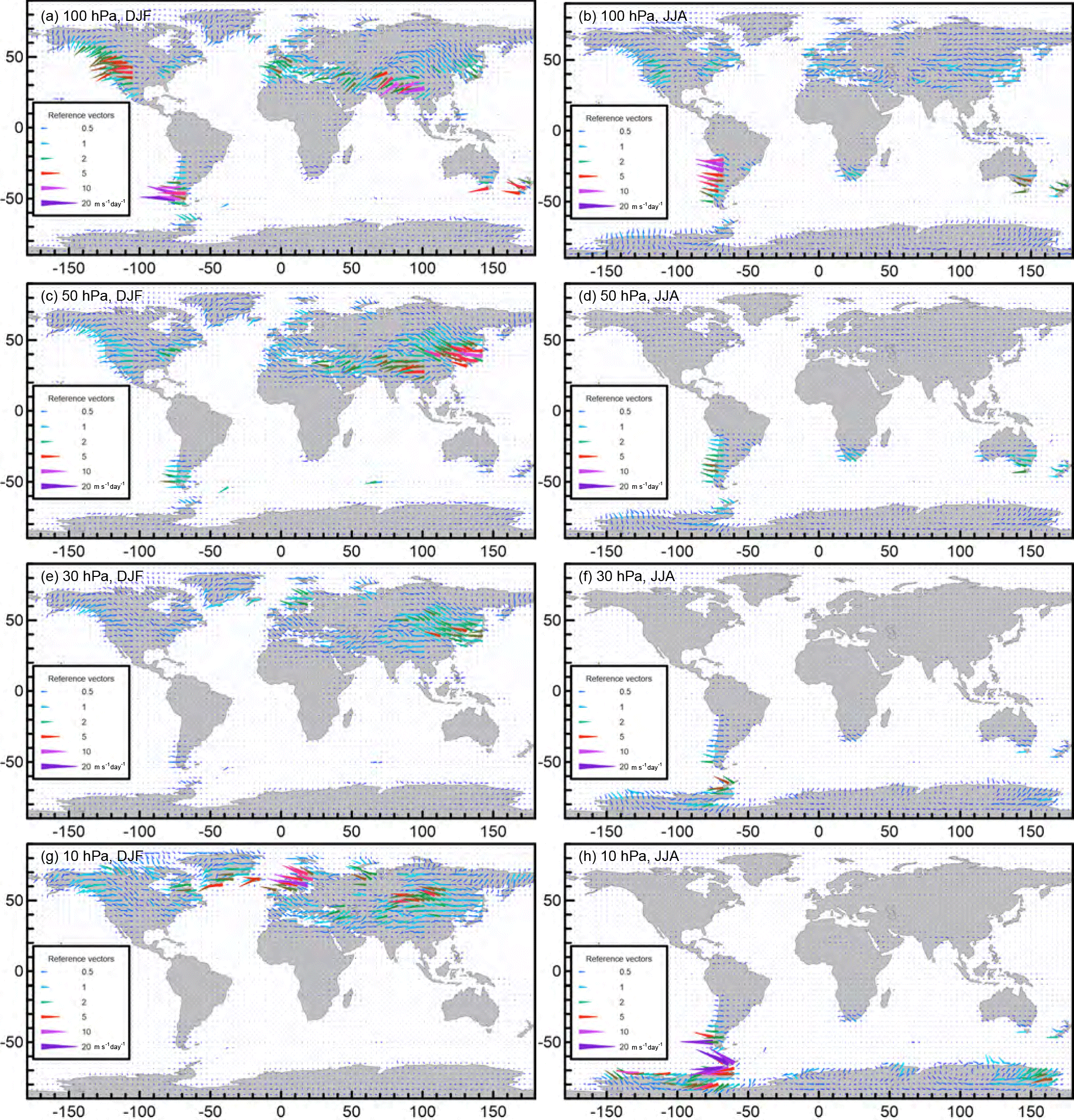
Figure 1Mean seasonal wind tendency due to OGWs (m s⁻¹ day⁻¹) at the 100 hPa (a, b), 50 hPa (c, d), 30 hPa (e, f) and 10 hPa (g, h) level, during DJF (a, c, e, g) and JJA (b, d, f, h) seasons.

Download

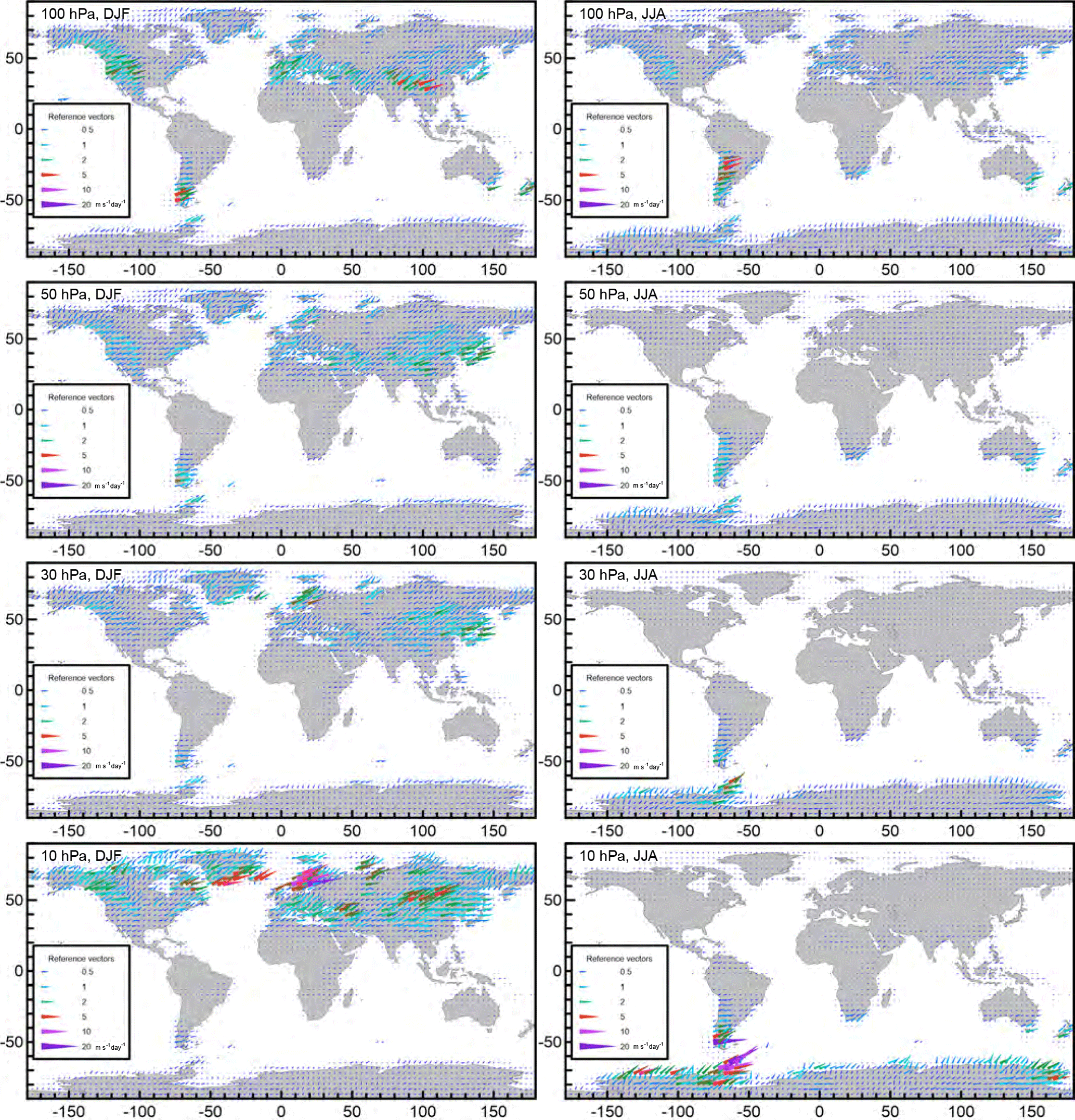
Figure 2Standard deviation (SD) of the monthly series of wind tendency due to OGW (m s⁻¹ day⁻¹), displayed in a vector-like form and assigning the value for the eastward component to the x axis and value for the northward component to the y axis.

Download

In the JJA season at 100 hPa, there is no dominant hotspot in the NH, while the SH OGWD distribution is dominated by the hotspot connected to the Andes. At 50 hPa in the DJF, there is a dominating hotspot in the region of eastern Asia corresponding to the eastern Asia/northern Pacific (EA/NP) hotspot observed by Šácha et al. (2015) or referred to as Mongolian orography in White et al. (2017, 2018). In the SH in the JJA season, the Andes are dominant, but note that the OGWD magnitude is smaller than for the EA/NP in the DJF season. Interestingly, at 30 hPa we see the dominance of the same hotspots as at 50 hPa but with a smaller magnitude of OGWD. In the SH in the JJA, the OGWD around the Drake Passage and Antarctic Peninsula (Hindley et al., 2015; Hoffmann et al., 2013, 2016; Wright et al., 2016b; de la Torre et al., 2012) begins to gain strength. At 10 hPa, in the NH in DJF, the Scandinavian hotspot starts to be dominant (Hoffmann et al., 2013; John and Kumar, 2012). In the SH in JJA, the southern Andes (Hoffmann et al., 2013; de la Torre et al., 2012), Drake Passage and Antarctic Peninsula hotspots dominate. Interestingly, we can also see moderately strong OGWD (Fig. 1c, 50 hPa, DJF) over small remote islands in the SH (Alexander and Grimsdell, 2013; Hoffmann et al., 2013). We conclude that the OGWD distribution from CMAM-sd gives a sufficiently realistic distribution of the OGWD for our analysis, given the assumptions employed in the parameterization and the lack of direct observational information on the OGWD and GWD in general.

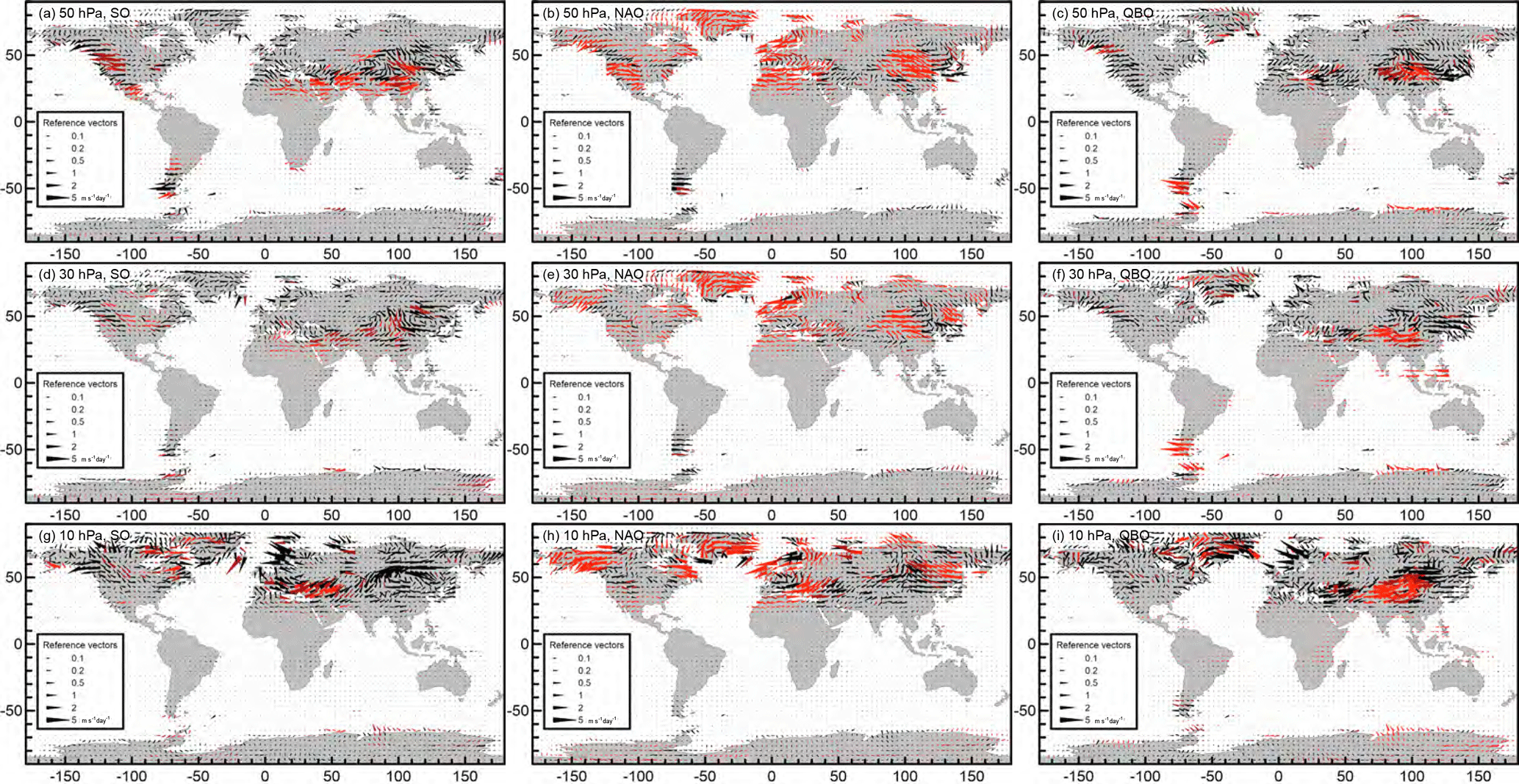
Figure 3Response of the OGWD (m s⁻¹ day⁻¹) at the 50 hPa (a, b, c), 30 hPa (d, e, f) and 10 hPa (g, h, i) level related to the activity of the Southern Oscillation (a, d, g), North Atlantic Oscillation (b, e, h) and quasi-biennial oscillation (c, f, i). The responses correspond to the increase in the oscillation index by four times its SD, i.e., to the transition of the respective oscillation from a highly negative to a highly positive phase; red symbols pertain to locations with at least one wind tendency component response statistically significant at the 95 % confidence level; bright red indicates at least one component significant at the 99 % confidence level. Analysis period: 1979–2010, monthly data, DJF season.

Download

Figure 2 gives an illustration of how much the OGWD is changing on the interannual scale. Note that the arrows do not show the drag direction but illustrate a ratio of the meridional and zonal SD (both always positive). We see that at 10 hPa, large OGWD variations correspond to Scandinavia, central Asia and Greenland in the NH and the southern tip of the Andes together with the region of Antarctic Peninsula in the SH winter. standard deviation (SD) values reach 20 m s⁻¹ day⁻¹ in both hemispheres with a prevalence of the zonal OGWD component (except the Antarctic Peninsula). The OGWD variability at the 30 hPa level is dominated by the EA/NP and Scandinavian hotspots with maximum values of SD below 5 m s⁻¹ day⁻¹. This magnitude is reached only in the Antarctic Peninsula region in JJA in the SH. In the NH, the meridional component has relatively lower variability than at 10 hPa.

At 50 hPa in the NH winter, we see the largest OGWD variations in the EA/NP hotspot and surprisingly large values also locally in the SH in the southern Andes. This is also the only region with pronounced variation in OGWD in the SH winter. The Rocky Mountains and especially the Himalayas and southern Andes with SD values around 5 m s⁻¹ day⁻¹ dominate the 100 hPa level in DJF. At 100 hPa, the relative contribution of the meridional OGWD component variability is bigger than at 50 and 30 hPa. In SH in DJF and JJA, the variability in the Andes dominates.

Figure 4Response of the OGWD (m s⁻¹ day⁻¹) at the 50 hPa (a, b, c), 30 hPa (d, e, f) and 10 hPa (g, h, i) level related to the activity of the Southern Oscillation (a, d, g), North Atlantic Oscillation (b, e, h) and quasi-biennial oscillation (c, f, i). The responses correspond to the increase in the oscillation index by 4 times its SD, i.e., to the transition of the respective oscillation from a highly negative to a highly positive phase; red symbols pertain to locations with at least one wind tendency component response statistically significant at the 95 % confidence level; bright red indicates at least one component significant at the 99 % confidence level. Analysis period: 1979–2010, monthly data, JJA season

Download

Generally, the OGWD varies interannually by about half of the climatological OGWD magnitude (even reaching it at 10 hPa), with respective hotspots dominating the variability at the particular pressure levels of their climatological influence.

3.2 MLR results

Responses of the OGWD to the phase of major internal climate oscillations are shown at the 50, 30 and 10 hPa levels. In the NH in DJF, the variability connected with NAO dominates by far (Fig. 3, middle column) in the sense that it is distributed across the whole hemisphere with many significant regions and responses of up to 5 m s⁻¹ day⁻¹. As could be expected from the NAO definition, it is most pronounced in regions surrounding the North Atlantic. Note especially that at all analyzed isobaric levels, there is a dipole-like structure between Greenland and Scandinavia together with coastal areas in other places in western Europe. That indicates that during the positive NAO phase the GW activity suppresses the eastward wind above Greenland and enhances it above western Europe while the opposite is true of the negative phase. A similar dipole can be found at the western coast of North America, but only at the 50 hPa level. At higher levels, the signal above Alaska is more pronounced. The NAO signal is also pronounced in northeastern America, central Asia and partly in the EA/NP region (at 50 and 30 hPa levels) and in northern Asia for the 10 hPa level. There is also a significant signal exceeding 2 m s⁻¹ day⁻¹ in northern Africa for the 50 hPa level. The SO signal in the DJF season in the NH is mostly pronounced at 50 and 10 hPa level. At 50 hPa it constitutes a ring of significant OGWD responses higher than 2 m s⁻¹ day⁻¹, whereas at the 10 hPa level the signal in northeastern America, Turkey, Iran and the Caucasus region dominates. At 50 hPa there is also a strong localized signal in the southern tip of South America. The QBO signal in DJF is mostly pronounced in central Asia in the NH and southern Andes together with the Antarctic Peninsula at 50 and 30 hPa in the SH.

During austral winter (JJA; Fig. 4), the largest signal found in the OGWD belongs to the SO, with Antarctica dominating at the 50 hPa level. At higher levels there is a dipole-like feature between Antarctica and the southern tip of the Andes. There is also a strong (more than 2 m s⁻¹ day⁻¹) significant signal connected with the QBO at the 50 hPa level over the Andes. Somewhat surprisingly we can also find a significant NAO signal (ca. 1 m s⁻¹ day⁻¹) around southern Australia and New Zealand at 50 hPa. The results of the regression of solar activity and volcanic forcing were not shown because they gain a mostly insignificant OGWD signal. Only at 50 hPa is there a weak (up to 1 m s⁻¹ day⁻¹) significant solar signal in northeastern America and Antarctica in their respective winter periods.

To illustrate that it is necessary to consider geographical distribution for the analysis of the interannual variability in OGWD, we show the MLR results also for zonal means of OGWD (shown for DJF only). For the zonal OGWD component (Fig. 5), we can see that there is only a weak positive significant NAO signal at all levels and a very small positive significant SO signal at 50 hPa between 20–30^∘ N corresponding to the belt described in the discussion of the Fig. 3. The magnitude of the detected signal is lower than 1 m s⁻¹ day⁻¹ everywhere. For the QBO and also for the meridional component (Fig. 6) of all indices, the signal is not significantly positive or negative or lower than 0.1 m s⁻¹ day⁻¹ almost anywhere. The situation is similar also for the JJA season (not shown).

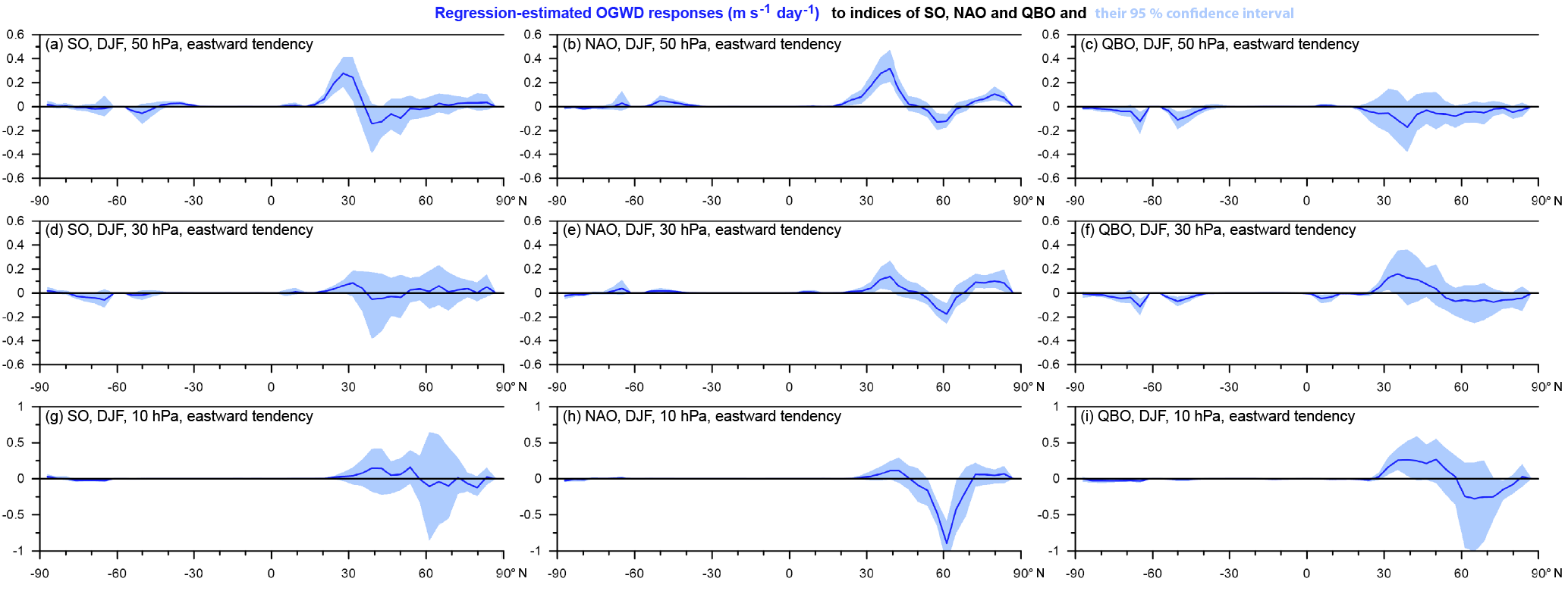
Figure 5Response of the zonal-mean OGWD (m s⁻¹ day⁻¹) at the 50 hPa (a, b, c), 30 hPa (d, e, f) and 10 hPa (g, h, i) level related to the activity of the Southern Oscillation (a, d, g), North Atlantic Oscillation (b, e, h) and quasi-biennial oscillation (c, f, i). The responses correspond to the increase in the oscillation index by 4 times its SD, i.e., to the transition of the respective oscillation from a highly negative to a highly positive phase; the blue curve shows the signal value and blue shading illustrates the 95 % confidence interval. Analysis period: 1979–2010, monthly data, DJF season.

Download

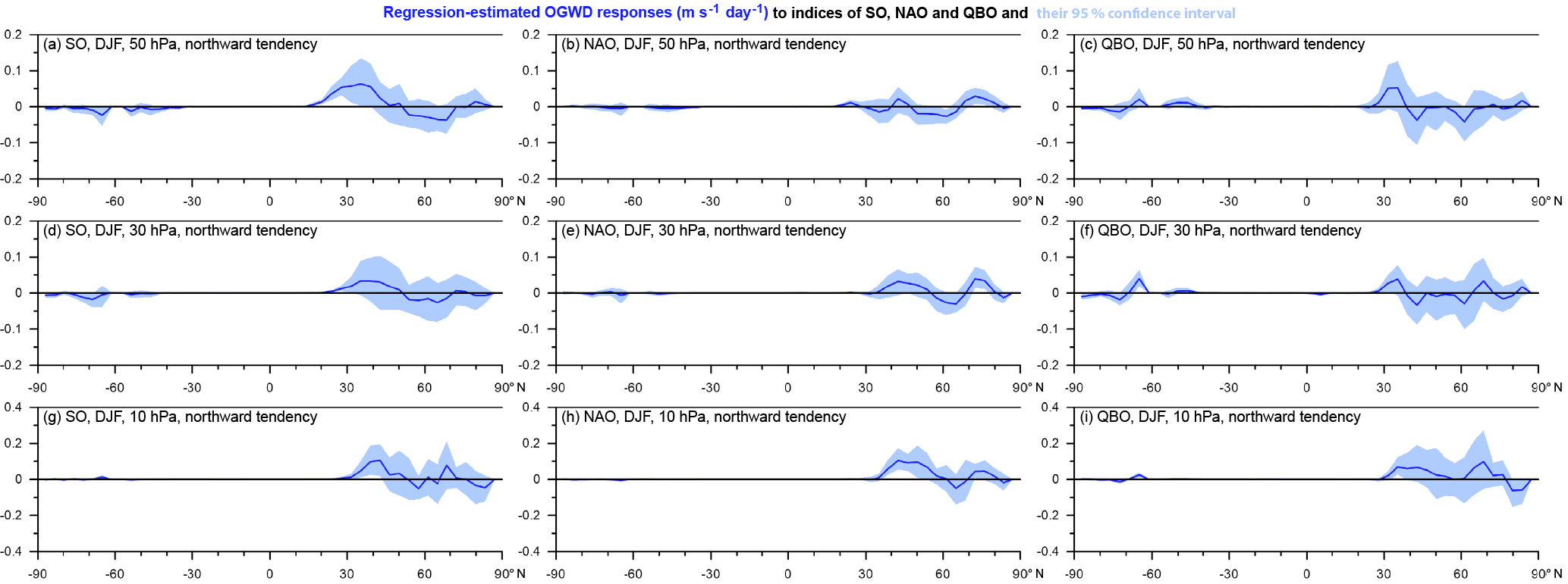
Figure 6Response of the meridional mean OGWD (m s⁻¹ day⁻¹) at the 50 hPa (a, b, c), 30 hPa (d, e, f) and 10 hPa (g, h, i) level related to the activity of the Southern Oscillation (a, d, g), North Atlantic Oscillation (b, e, h) and quasi-biennial oscillation (c, f, i). The responses correspond to the increase in the oscillation index by 4 times its SD, i.e., to the transition of the respective oscillation from a highly negative to a highly positive phase; the blue curve shows the signal value and blue shading illustrates the 95 % confidence interval. Analysis period: 1979–2010, monthly data, DJF season.

Download

The general finding of the results presented above is that the OGWD varies locally by a few meters per second per day depending on the phase of the climate indices and also that the geographical variation in hotspots can vary from a phase to phase. The analysis also points to the important finding that the significant signal connected to the climate oscillations diminishes in the case of the traditional zonal-mean approach.

3.3 Explanatory factors

The results presented above alone cannot confirm our hypothesis on the tropospheric variability transfer to the stratosphere by altering the GW activity and its distribution because the MLR results do not illustrate the causality of the problem considered. It can be argued that the OGWD variability results are caused simply by the variations in the stratosphere or upper troposphere (e.g., jet shift, meandering due to anomalous planetary wave (PW) activity) possibly leading to Doppler shifting effects or variations in critical lines for the orographic GW propagation (Pisoft et al., 2018). The modulation of GWs by PWs receives great attention in the scientific community (Cullens et al., 2015), and considering this causality mechanism, the dynamical influence of the OGWD variations would be of secondary importance only. Therefore, in this subsection we analyze the daily data of wind direction and speed (the influence of another OGWD parameterization variable – a stability – was not diagnosed) to show that at least a part of the OGWD variability is directly influenced by the variability at the surface or in the lower troposphere.

Figures 7, 8 and 9 present an analysis of daily data aimed at estimating how much of the OGWD variability at a given level can be explained by 850 hPa wind variance. At 50 hPa, we can see that the link between the lower-tropospheric winds and OGWD is strongly expressed in a belt in the midlatitudes and tropics of the NH. The fraction of variance explained is maximal and the geographical distribution is also very similar for the links between zonal wind/the zonal OGWD component and meridional wind/the meridional OGWD component. In the regions with significant orography and particularly in the region of the EA/NP hotspot (which dominates the OGWD field at 50 hPa in the NH), the majority of OGWD variance is explained by lower-tropospheric winds.

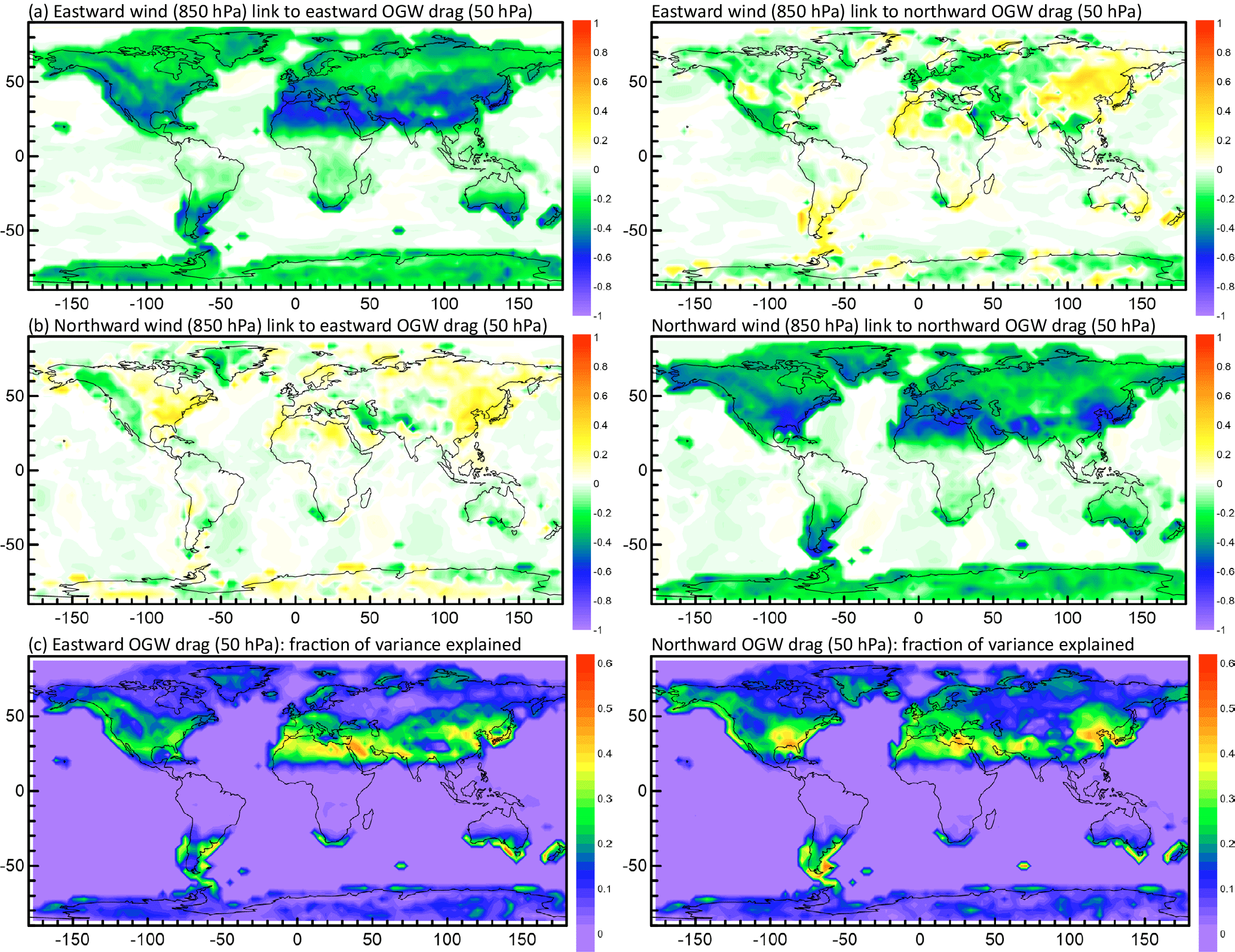
Figure 7(a, b) Standardized regression coefficients between orographic gravity wave drag at the 50 hPa level (predictand) and eastward and northward wind components at the 850 hPa level (predictors), during the DJF season. (c) Coefficient of determination, i.e., the fraction of total variance of OGWD explained through the regression mappings by both components of wind at the 850 hPa level. Analysis period: 1979–2010, daily data, DJF season.

Download

Figure 8(a, b) Standardized regression coefficients between orographic gravity wave drag at the 30 hPa level (predictand) and eastward and northward wind components at the 850 hPa level (predictors), during the DJF season. (c) Coefficient of determination, i.e., the fraction of total variance of OGWD explained through the regression mappings by both components of wind at the 850 hPa level. Analysis period: 1979–2010, daily data, DJF season.

Download

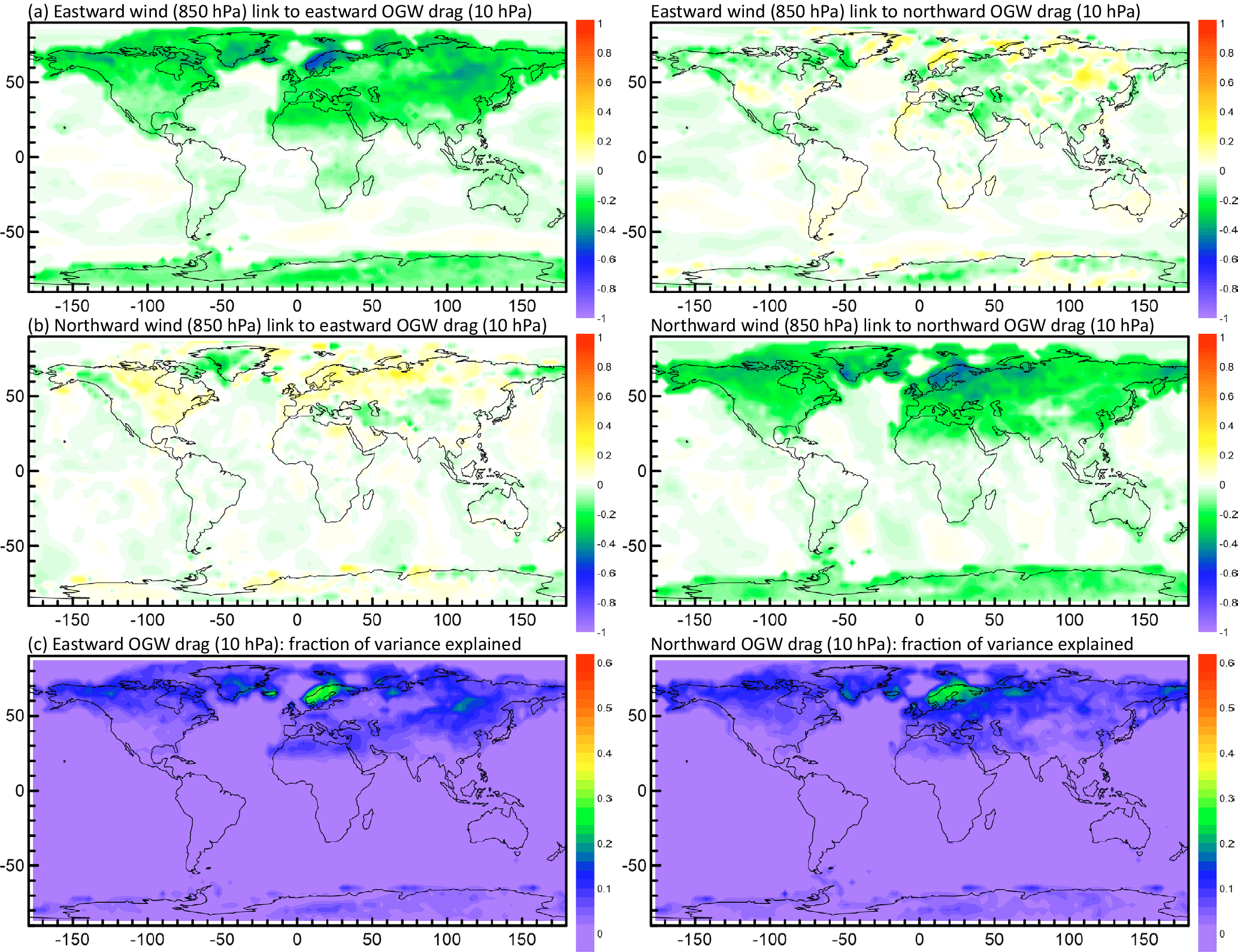
Figure 9(a, b) Standardized regression coefficients between orographic gravity wave drag at the 10 hPa level (predictand) and eastward and northward wind components at the 850 hPa level (predictors), during the DJF season. (c) Coefficient of determination, i.e., the fraction of total variance of OGWD explained through the regression mappings by both components of wind at the 850 hPa level. Analysis period: 1979–2010, daily data, DJF season.

Download

An interesting pattern can be seen in the SH around the Andes, where the maximum of the OGWD variance explained is located up- and downwind from the Andes. Also interestingly, at 50 hPa, in the southern Andes/Antarctic Peninsula region, a larger fraction of the meridional OGWD component variance is explained by surface conditions than for the zonal component. Otherwise, the fraction of the OGWD variability explained in the Australian/New Zealand hotspot (connected in previous analyses mainly with the NAO signal) is about two-fifths of the total variance.

At the 30 hPa level the fraction of variance explained is lower – around one-third of the variance in eastern Asia and locally in northern Atlantic coastal regions and in the SH. In the eastern Asia region this is due to the stratospheric background affecting the critical line occurrence and propagation of the GWs between 50 and 30 hPa. Interestingly, for the meridional OGWD component, the fraction of variance explained is slightly higher. At the 10 hPa level, there is a single maximum of explained total variance (around one-third) in Scandinavia. A similar amount of variance is also explained by 850 hPa winds for Iceland but for the zonal OGWD component only.

Another approach allowing us to assess the variability in the orographic GW sourcing is to analyze the 850 hPa orographic GW fluxes as a proxy and apply the MLR method. However, with this method it is not possible to link the results directly with the variability in the OGWD because processes like the Doppler shifting of amplitudes or critical line variations can alter the resulting OGWD significantly. Also note, that this analysis is made with monthly data and the comparability with previous analyses is limited.

In Fig. 10 we see that in the NH in DJF there is a strong signal in Greenland and western Europe connected with the NAO and an equally strong signal in GW sourcing variability in central Asia (Himalayas), Greenland, Iceland and Svalbard connected with the QBO. The SO signal is largely insignificant in the NH, but in the SH in JJA it is most strongly pronounced mainly in the southern tip of the Andes and Antarctic Peninsula. In the SH in JJA, some regions of significant signal in GW sourcing variability connected with the NAO (the Andes, Australia and New Zealand) and QBO (Antarctica) can also be found.

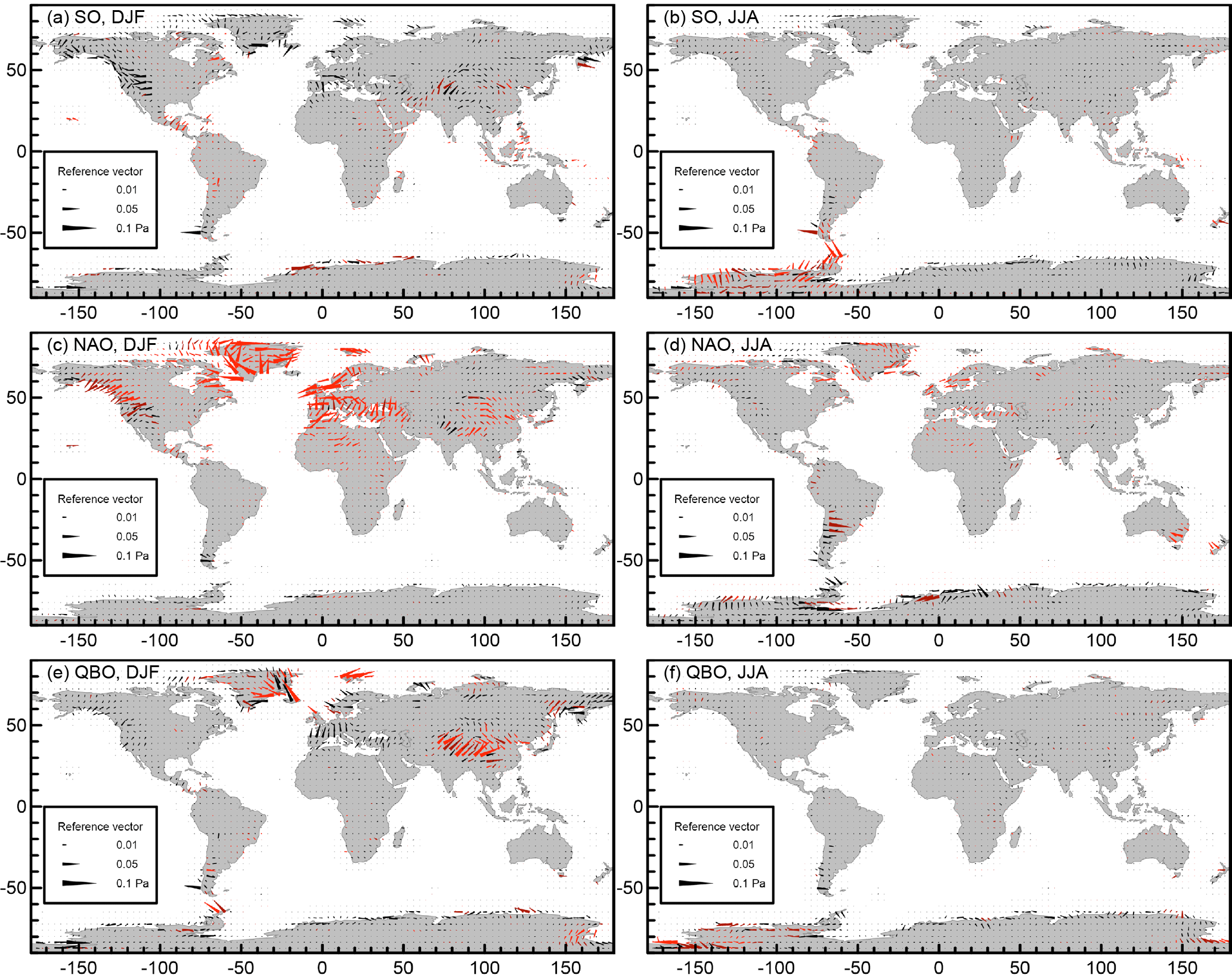
Figure 10Response of the orographic GW momentum fluxes (Pa) at the 850 hPa level related to the activity of the Southern Oscillation (a, b), North Atlantic Oscillation (c, d) and quasi-biennial oscillation (e, f) during DJF (a, c, e) and JJA (b, d, f) seasons. The responses correspond to the increase in the oscillation index by 4 times its SD, i.e., to the transition of the respective oscillation from a highly negative to a highly positive phase; red symbols pertain to locations with at least one orographic GW flux component response statistically significant at the 95 % confidence interval. Analysis period: 1979–2010, monthly data.

Download

Although the strong QBO signal may be surprising, the QBO phase exhibits a distinct and in some regions statistically significant influence on the lower-tropospheric winds in CMAM-sd (not shown). The influence of the QBO on the surface meteorological conditions has been pointed out in the literature in detail before (Hansen et al., 2016; Marshall and Scaife, 2009).