2.1 Data

The target region in this study comprises the AR (Fig. 1a) as defined by Roberts et al. (2010) and used by Vázquez et al. (2016), the AO as a whole, and its 13 main subdomains as defined in Fig. 1b (Boisvert et al., 2015). The analysed period was from 1 January 1980 to 31 December 2016. For Arctic SIE, we used daily, monthly, and annual data from the US National Snow and Ice Data Center (Fetterer et al., 2016). To implement the Lagrangian approach, by which moisture transport is estimated to approximate vertical integrated moisture fluxes and circulation types, we used the European Centre for Medium-Range Weather Forecasts (ECMWF) ERA-Interim reanalysis (Dee et al., 2011). Data from this reanalysis cover the period from January 1979 to the present and extending forward continuously in near-real time. These data are available at 6 h intervals at a 1^∘ × 1^∘ spatial resolution in latitude and longitude for 61 vertical levels (1000 to 0.1 hPa). The ERA-Interim reanalysis is typically considered to have the highest quality relative to other reanalysis data for the water cycle (Lorenz and Kunstmann, 2012) and is especially appropriate over the AR (Jakobson et al., 2012), with better representation of mass fluxes including water vapour (Graversen et al., 2011).

2.2 Methods

2.2.2 Detection of change points in Arctic sea ice extent

We have used several methods to estimate CPs in Arctic SIE. As usual in time series analysis a CP detection tries to identify times when the time series in mean or variance changed; in this case we were interested mainly in changes in mean. Changes in mean for the Arctic SIE are equivalent to a decrease, higher Arctic SIE values before the CP and lower after it.

CPs of each of these series for the AO were calculated using three different methods, one detecting single CPs (at most one change, AMOC) and two detecting multiple CPs (binary segmentation, BinSeg; and pruned exact linear time, PELT).

AMOC uses a test to detect a hypothesised single CP. The null hypothesis refers to no CP, and its maximum log likelihood is given by $\log p\left(y_{\mathrm{1}:n}\mathrm{|}\widehat{{\mathit{\theta }}_{\mathrm{1}}}\right)$, where p(⋅) is the probability density function associated with the distribution of the data and $\widehat{\mathit{\theta }}$ is the maximum likelihood estimate of the parameters. For the alternative hypothesis, a CP at τ₁ is considered, with ${\mathit{\tau }}_{\mathrm{1}}\in \left\{\mathrm{1},\mathrm{2},\mathrm{\dots },n-\mathrm{1}\right\}$. The expression for the maximum log likelihood for a given τ₁ is ML$\left({\mathit{\tau }}_{\mathrm{1}}\right)=\log p\left(y_{\mathrm{1}:{\mathit{\tau }}_{\mathrm{1}}}\mathrm{|}\widehat{{\mathit{\theta }}_{\mathrm{1}}}\right)+\log p\left(y_{({\mathit{\tau }}_{\mathrm{1}}+\mathrm{1}):n}\mathrm{|}\widehat{{\mathit{\theta }}_{\mathrm{2}}}\right)$.

Taking into account that the CP location is discrete in nature, maxτ₁ML(τ₁) is the maximum log-likelihood value under the alternative hypothesis, where the maximum is taken over all possible CP locations. Consequently, the test statistic is $\mathit{\lambda }=\mathrm{2}\left[max{\mathit{\tau }}_{\mathrm{1}}\mathrm{ML}\left({\mathit{\tau }}_{\mathrm{1}}\right)-\log p\left(y_{\mathrm{1}:n}\mathrm{|}\widehat{\mathit{\theta }}\right)\right]$. The null hypothesis is rejected if λ > C, where C is a threshold of our choice. When detecting a CP, its position is estimated as $\widehat{{\mathit{\tau }}_{\mathrm{1}}}$, which is the value of $\widehat{{\mathit{\tau }}_{\mathrm{1}}}$ that maximises ML(τ₁).

BinSeg and PELT function as follows: by summing the likelihood for each of the m segments, the likelihood test statistic can be extended to multiple changes. However, there is a problem in identifying the maximum of ML(τ_1:m) over all possible combinations of τ_1:m. The most common approach to resolve this problem is to minimise

$$\begin{array}{}\text{(1)}& \sum _{i=\mathrm{1}}^{m+\mathrm{1}}\left[C\left(y_{\left({\mathit{\tau }}_{i-\mathrm{1}}+\mathrm{1}\right):{\mathit{\tau }}_i}\right)\right]+\mathit{\beta }f\left(m\right),\end{array}$$

where C is a cost function for a segment, such as the negative log likelihood, and βf(m) is a penalty to guard against over-fitting. The BinSeg method starts with applying a single CP test statistic to the entire data set. If a CP is identified, the data are then split into two at the CP location. The single CP process is repeated for the two new data sets, before and after the change. If CPs are identified in either of the new data sets, they are split further. This procedure continues until no CPs are found in any parts of the data. This process is an approximate minimisation of Eq. (1) with f(m)=m, as any CP locations are conditional on CPs identified previously. The segment neighbourhood algorithm precisely minimises the expression given by Eq. (1) using a dynamic programming technique to obtain the optimal segmentation for (m+1) CPs reusing the information calculated for m CPs. The PELT method is similar to that of the segment neighbourhood algorithm in that it provides an exact segmentation. We have used the PELT algorithm instead of the segment neighbourhood method as it has proven to be more computationally efficient. The reason for this greater efficiency is the use of dynamic programming and pruning in the algorithm's construction.

A full description of these methods and the subroutines in R used in this study can be found in Killick and Eckley (2014).

The three different CP detection methods were used for the four different Arctic SIE time series defined in Sect. 2.2.1. Figure 2 illustrates the detection of the CP in mean for two series (ADS and AMS) using the AMOC method. The top plot represents the 13 505-value Arctic ice extent anomaly series consisting of all days from 1 January 1980 to 31 December 2016 (ADS series). There are two horizontal lines representing the mean of the values before and after the CP identified by the AMOC method (the 8660th day that corresponds to 22 September 2003). Those means are 0.27 and −0.91 million km², respectively. The graphic at the bottom portrays the 444-value Arctic ice extent anomaly series consisting of all months from January 1980 to December 2016 (AMS series). As in the previous one, there are two horizontal lines, which correspond to the SIE mean before and after the AMOC CP (the 286th month of the series, that is October 2003). Those means are 0.41 and −0.74 million km², respectively.

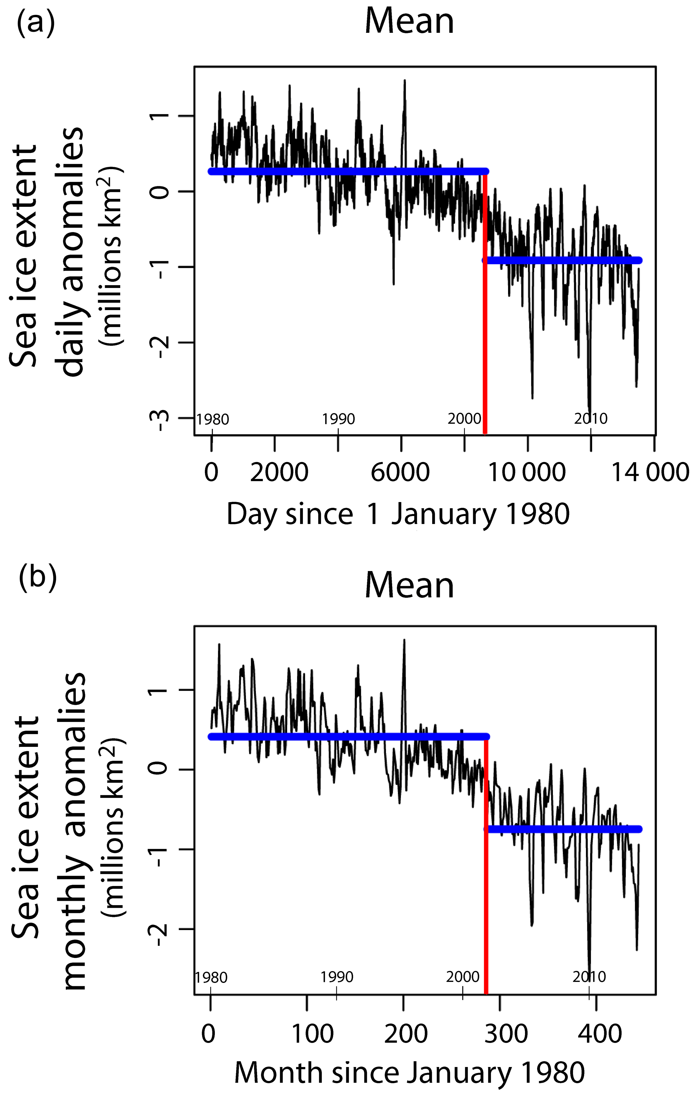
Figure 2Example of change point detection in mean for two series and one method, AMOC. Panel (a) represents the change points in the ADS series. The two horizontal lines represent the mean of the values before and after the change point identified with the AMOC method (8660th day – 22 September 2003). Those means are 0.27 and −0.91 million km², respectively. Panel (b) represents the change points in the AMS series. The two horizontal lines represent the mean of the values before and after the change point identified with the AMOC method (286th month – October 2003). Those means are 0.41 and −0.74 million km², respectively.

Download

2.2.3 Estimation of the Lagrangian moisture transport from the main sources

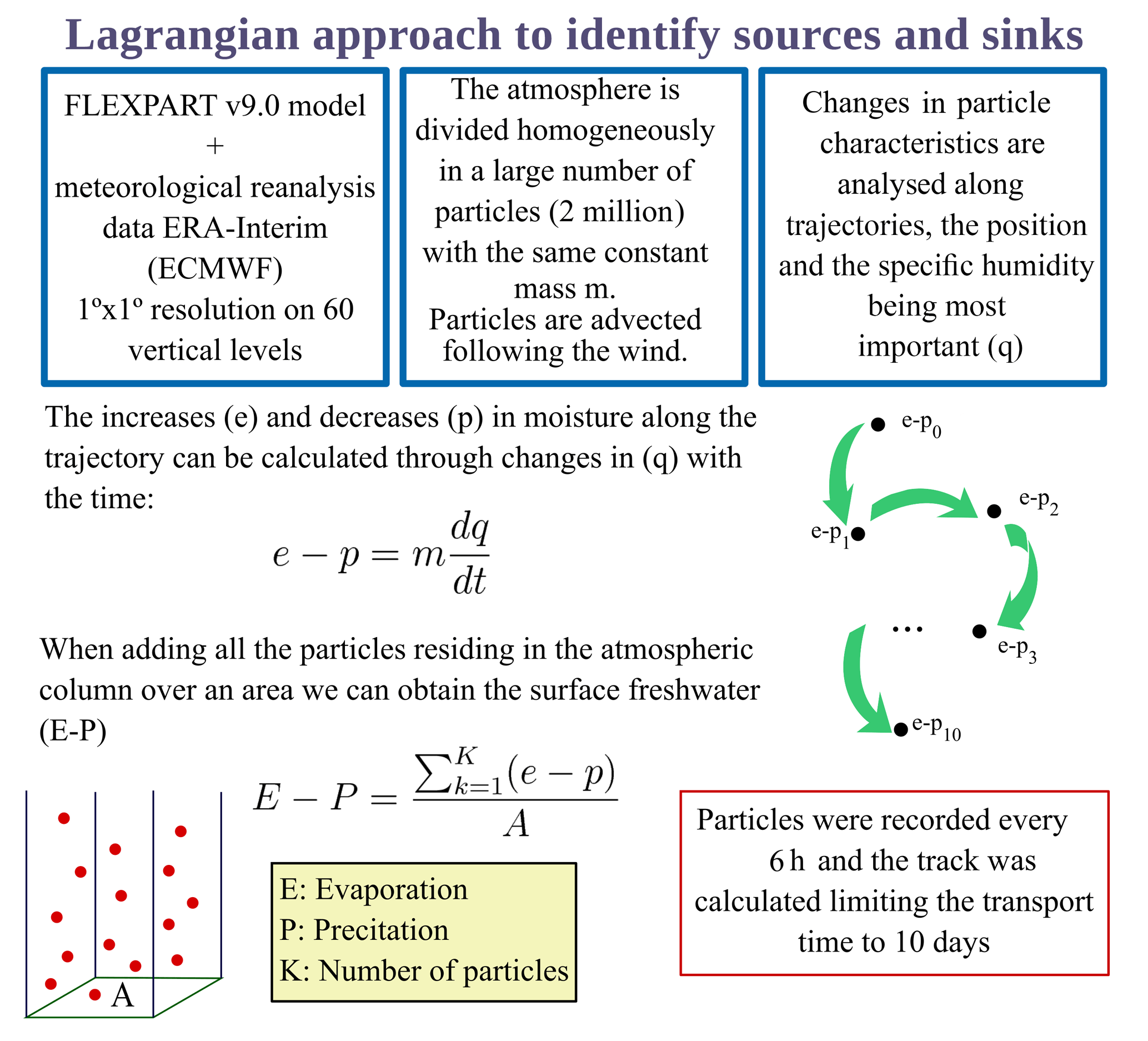
In this study, we used a Lagrangian approach to calculate moisture transport from the main moisture sources as detected by Vázquez et al. (2016) (Fig. 1c) for the AR, AO, and its 13 subregions. This approach is based on the particle dispersion model FLEXPART v9.0 (i.e. the FLEXible PARTicle dispersion model of Stohl and James, 2004, 2005) forced by ERA-Interim data from the ECMWF. This approach has been used extensively in moisture transport analysis (e.g. Gimeno et al., 2010, 2013), and a review of its advantages and disadvantages versus other approaches for tracking water vapour was summarised by Gimeno et al. (2012 and 2016). To briefly summarise this method, the atmosphere is divided into so-called particles (finite elements of volume with equal mass) and individual three-dimensional trajectories are tracked backward or forward in time for 10 days, the average residence time of water vapour in the atmosphere (Numaguti, 1999). Then, taking into account the changes in (q) for each particle along its trajectory, the net rate of change of water vapour (e−p) for every particle, $(e-p)=m(\mathrm{d}q/\mathrm{d}t)$, is estimated, with e and p representing evaporation and precipitation, respectively. The total atmospheric moisture budget (E−P) is estimated by adding up (e−p) for all particles over a given area at each time step used in the analysis. If we follow the particles backward in time for a target region, positive (E−P) values identify the main moisture sources for this target region; if we follow the particles forward in time from a source region, negative (E−P) values identify the main moisture sinks of the source region. In this study we have used four predefined moisture sources, those identified as the major sources of moisture for the AR in Vázquez et al. (2016) following all the particles reaching the AR for the period 1980–2012 backward in time and taking the regions showing positive (E−P) values greater than the 90th percentile (taking into account global values of positive E−P). Then, to compute MTP from each of these four sources to each sink for the AO, the trajectories of particles from the moisture sources for the AR were followed forward in time from every source region detected by Vázquez et al. (2016) (Fig. 1c). This was carried out for 6 h in the period 1980–2016. Then, we selected all particles losing moisture, (e−p) < 0, at the sinks (the whole Arctic or any of the subregions), and by adding e−p for all of these particles, we estimated moisture transport for precipitation from the source to the sink ((E−P) < 0) at daily, monthly, or yearly scales. A schematic illustration of this approach is displayed in Fig. 3. A couple of clarifications on this approach are necessary to avoid misunderstandings of the results. The first one is that particles can gain moisture in the regions placed between those defined as the major moisture sources and the target region, even in the target region itself. However as our defined moisture regions were identified as the major moisture sources in the backward analysis (Vázquez et al., 2016) the contribution of the intermediate regions is much lower. A look at Fig. 2 from Vázquez et al. (2016) shows that intermediate regions are not net sources (particles reaching the Arctic region lost (not gained) moisture in these regions on average). In any case not all the precipitated water comes from the major sources; those particles that were not within those major source regions 10 days before precipitation are responsible for the rest of precipitation, including the particles coming from the AR itself, which account for the important contribution of local moisture recirculation. The second clarification is concerned with the size of the target regions and the number of particles reaching them. As commented on in the seminal description of the approach (Stohl and James, 2004, 2005), it works better for large regions. The size of the target regions in this study (Arctic region and subregions) is bigger than in many of the regions where the same methodology was used in previous studies (e.g. Ramos et al., 2016 or Wegmann et al., 2015) and the average number of particles by source that reach the target regions high enough daily (see Table S1 in the Supplement).

Figure 3A scheme of the Lagrangian approach used to estimate moisture transport.

Download

3.1 Climatological moisture transport for precipitation to the Arctic region and Arctic Ocean subregions

Figure 4 displays the seasonal cycle of MTP to the AR from four major sources (Atlantic, Pacific, Siberia, and North America) and the relative contributions of each. MTP to the AR exhibits a marked seasonal cycle with a maximum in summer and a minimum in winter; MTP doubles in the highest month (August) relative to the lowest month (February). The percentage of the contribution from each source is relatively constant throughout the year, with the Pacific, North America, Siberia, and the Atlantic contributing about 35, 30, 20, and 15 %, respectively.

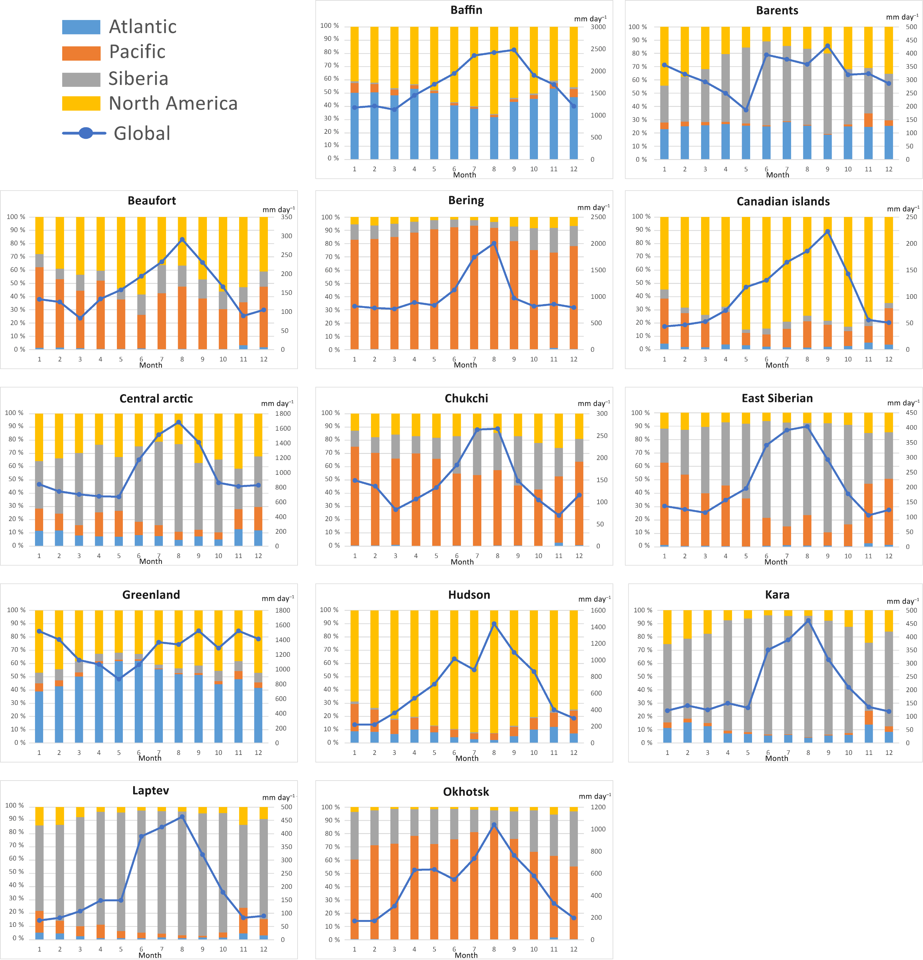
The seasonal cycle is quite similar for eight of the 13 AO subregions (Fig. 5), with two other regions (Barents and the central Arctic) exhibiting similar maxima, but with minima in May, and another (Chukchi Sea) with two minima in March and November, and finally Greenland with a minimum in May but no clear maximum in summer, extending the typical summer high values to autumn and winter. The relative contributions of each moisture source are very diverse, with three general patterns: one with the closest source dominating (a Pacific source for the Bering, Chukchi, and Okhotsk seas, a North American source for the Canadian Arctic Archipelago and Hudson Bay, and a Siberian source for the Kara and Laptev seas), another pattern in which two sources share importance throughout the year (Atlantic and Siberian sources for Baffin Bay and Greenland, and Pacific and North American sources for the Beaufort Sea), and a third in which the Siberian source shares importance with two or more sources (Barents Sea, central Arctic, and eastern Siberia).

Figure 4Seasonal cycle of moisture transport for precipitation (MTP) to the Arctic region (AR) from the four major sources (Atlantic, Pacific, Siberia, and North America). Values at the right represent absolute values of transport, and those at the left indicate the relative contribution of each source by percentage.

Download

Figure 5Same as in Fig. 3 but for each of the 13 subregions of the Arctic Ocean (AO).

Download

The relative importance of each ocean subregion for MTP to the AO (estimated as the sum of the 13 subregions) is shown in Fig. 6, where the percentage of moisture transport to the whole AO is displayed by region and month. There are four regions where the aggregated MTP received represents more than 60 % of the MTP received for the whole Arctic. Those regions are Greenland, Baffin Bay, the Bering Sea, and the central Arctic, in order of importance. The contributions of Baffin Bay, the Bering Sea, and the central Arctic vary little throughout the year, representing about 20, 12, and 10 % of the MTP received for the whole Arctic, respectively, whereas the contribution of Greenland has a marked seasonal cycle with values around 25 % for autumn and winter, and 10–15 % in spring and summer, seasons when two other sources gain importance, the Hudson Bay and Okhotsk Sea, with percentages close to 10 %. The almost constant contribution of the Barents Sea throughout the year is non-negligible, around 5 %. The remaining sources have contributions lesser than 5 %.

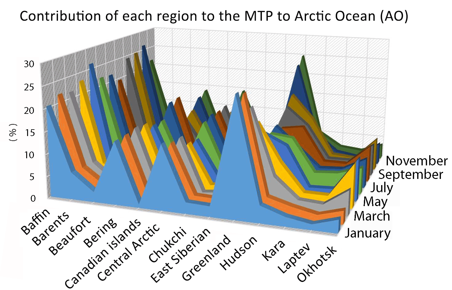
Figure 6Percentage of moisture transport for precipitation to the whole Arctic Ocean by subregion and month.

Download

3.2 Moisture transport after and before Arctic sea ice change points

Figure 7 summarises the identified CPs in means identified using the AMOC method in the four series of SIE anomalies (DS, MS, ADS, and AMS) from 1980 to 2016 for the whole Arctic.

Blue points refer to the CPs in DS; for instance, the 21 July daily anomaly series (size of the series: 37 data points, representing 37 annual anomalies of the values of the SIE for the 37 values on 21 July) occurred in 2004. DS only has CPs in the period from July to October. These CPs occurred mostly in 2004, the first part of September in 2006, and the last week of October in 2003. The results of both the BinSeg and PELT methods (results not shown) coincide for every day except for 17 September (2004 based on AMOC and 2006 for the other methods). The red bands in Fig. 7 portray the CPs in the MS data set (July–October). For instance, July monthly anomaly series (size of each series: 37 data points, representing 37 annual anomalies of the values of the SIE for the 37 values in the average monthly July) occurred in 2004. These CPs occurred in 2004 for July and September, a little earlier (2001) for August, and a little later (2005) for October. Both the BinSeg and PELT methods coincide in every month except for October (2005 based on AMOC and BinSeg, and 2006 for PELT). The single green square corresponds to the CP in the 13 505-value series consisting of all days from 1 January 1980 to 31 December 2016 (ADS). The CP occurred on 22 September 2003 and was identified by the BinSeg, although not by PELT (the closest ones are 4 August 2002 and 26 January 2005). The single purple line represents the CP in the 444-value series consisting of all months from January 1980 to December 2016 (AMS). This CP occurred in October 2003. The results of both the BinSeg and PELT methods coincide for this CP, and it is the only one for both. Overall, the results in Fig. 7 suggest that 2003 is the most appropriate year for analysis of differences in moisture transport after and before a single CP date. The average values for ADS before and after the CP were 0.27 and −0.91 million km² and for AMS 0.41 and −0.74 million km². The analysis of changes in MTP for the multiple subperiods identified by BinSeg and PELT would merit analysis, but it is out of the objective of this paper.

Figure 8 portrays the differences between mean values of MTP until 2003 and mean values after 2003 for every source region (Fig. 1c) for the AR, which includes continental and oceanic areas (Fig. 1a). The quantities in the plot result from averaging daily values of MTP. The statistical significance of the differences has been estimated by comparing daily values of MTP before and after the CP, and the sample size is large enough (30 × 23 years vs. 30 × 13 years) to permit application of Student's t test. The pattern of changes in MTP before and after the CP for the AR shows no significant changes in late winter and spring, a significant decrease in MTP in summer, and increased MTP in autumn and early winter, with the exception of October. The summer decrease is statistically significant for the contributions of Pacific and Siberian sources throughout the entire summer, for the Atlantic source in early summer, and for the North American source in late summer. The autumn–early winter increase is statistically significant (red asterisks) for the contributions of the North American source in three months (September, November, and December), for the Siberian and the Atlantic sources in two months (September and November and October and December, respectively), and for the Pacific source only in one month (November). As, according to Fig. 7 mainly for DS and MS, 2004 could also be interpreted as the main CP, we tested results of changes in MTP by changing 2003 by 2004 with almost identical results (not shown).

These results are coherent with any of the mechanisms referred in the introduction. Thus, (i) a lower MTP in early summer (as occurred since 2003) implies lower precipitation (in this season mainly as snowfall), which would result in a decrease in the surface albedo and thus increasing melt (Cheng et al., 2008); (ii) a lower MTP in late summer (as has occurred since 2003) could be due to a less probability of occurrence of rainfall storms with possible flooding over the ice, which would favour the formation of superimposed ice and consequently is consistent with increasing melt; (iii) a higher MTP in early autumn (September) (as has occurred since 2003) implies higher precipitation (in this season mainly as rainfall), something generally related to sea ice melt; (iv) a higher MTP in late autumn and early winter (as has occurred since 2003) implies higher precipitation (in this season mainly as snowfall), enhancing thermal insulation and thus reducing sea ice growth in (Leppäranta, 1993). The rigorous checking of these implications merits further analysis but it is out of the scope of this paper since it would imply knowing details over the precipitation form (snow or rain) for the different Arctic regions with good temporal and geographical resolution, and even to analyse specific precipitation episodes to know if these are responsible for flooding or not.

However, because Arctic ice cover is extensive in geographical domain covering the subregion affected by very different atmospheric circulation patterns, this pattern of change in MTP could be non-homogeneous for the entire AO and its subregions. Finer-scale analysis can be performed by restricting the analysis to oceanic areas only (the 13 AO subregions and the whole AO defined as the sum of these regions, Fig. 1b). The differences between mean values of MTP until 2003 and mean values after 2003 for every source region for the AO (Fig. 9 top left) is quite similar to the AR without significant changes in late winter and spring, with decreased MTP in summer and increased MTP in autumn and early winter, now also including October. Small differences are observed in the contributions of each source to the change of MTP toward the AO, with the Pacific source becoming much less important for the summer decrease and more important in the autumn increase. The consistent increment is especially remarkable after the CP of MTP for all the moisture sources in September, the month when Arctic SIE is lowest.

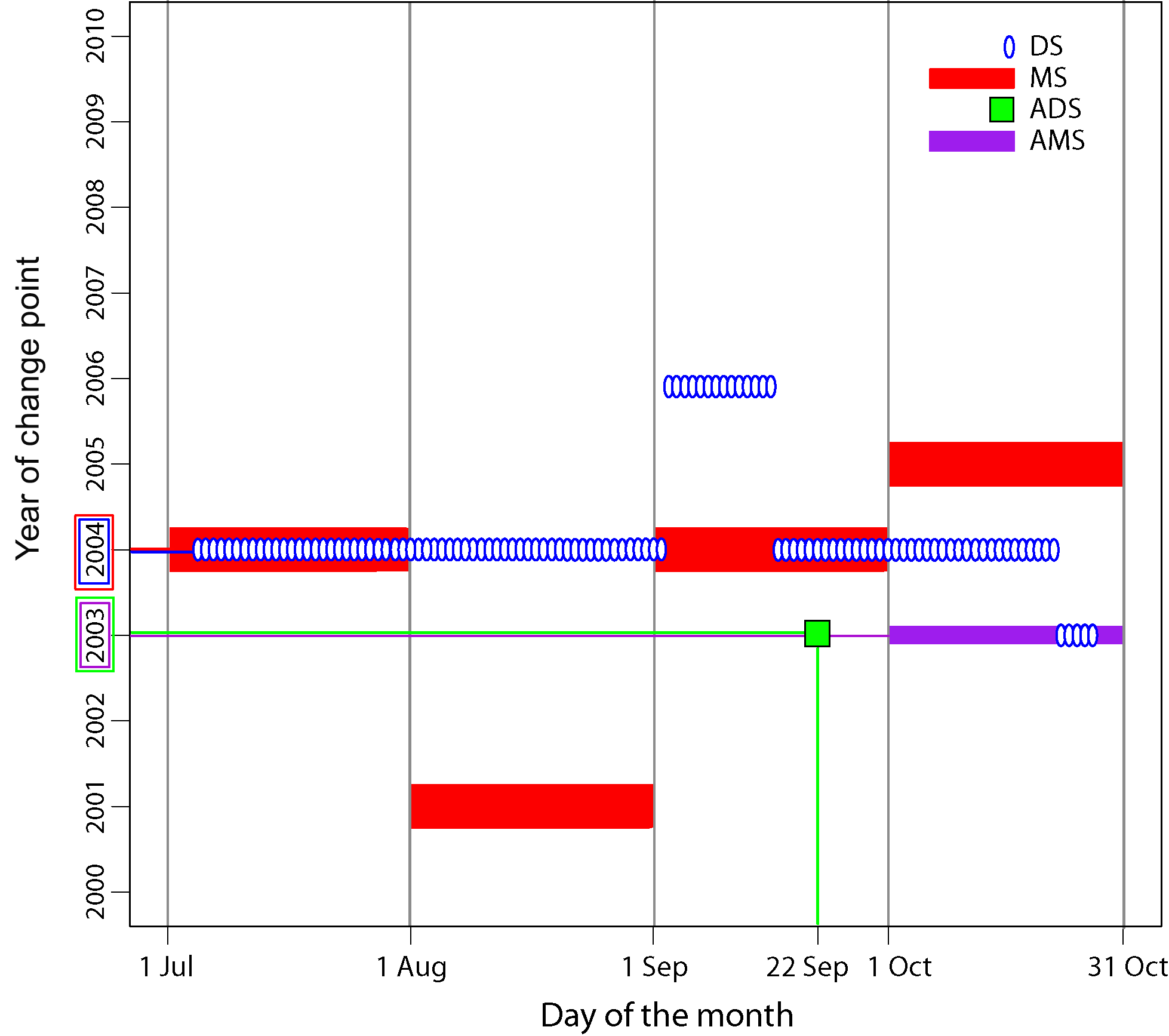
Figure 7Summary of the identified change points (CPs) in means identified using the AMOC method with the four series of ice extent anomalies for the whole Arctic (DS, MS, ADS, and AMS) from 1980 to 2016. The blue points refer to the change points in DS; the red lines portray change points in the MS (July–October). The green square corresponds to the change point in the ADS, and the purple line represents the change point in the AMS.

Download

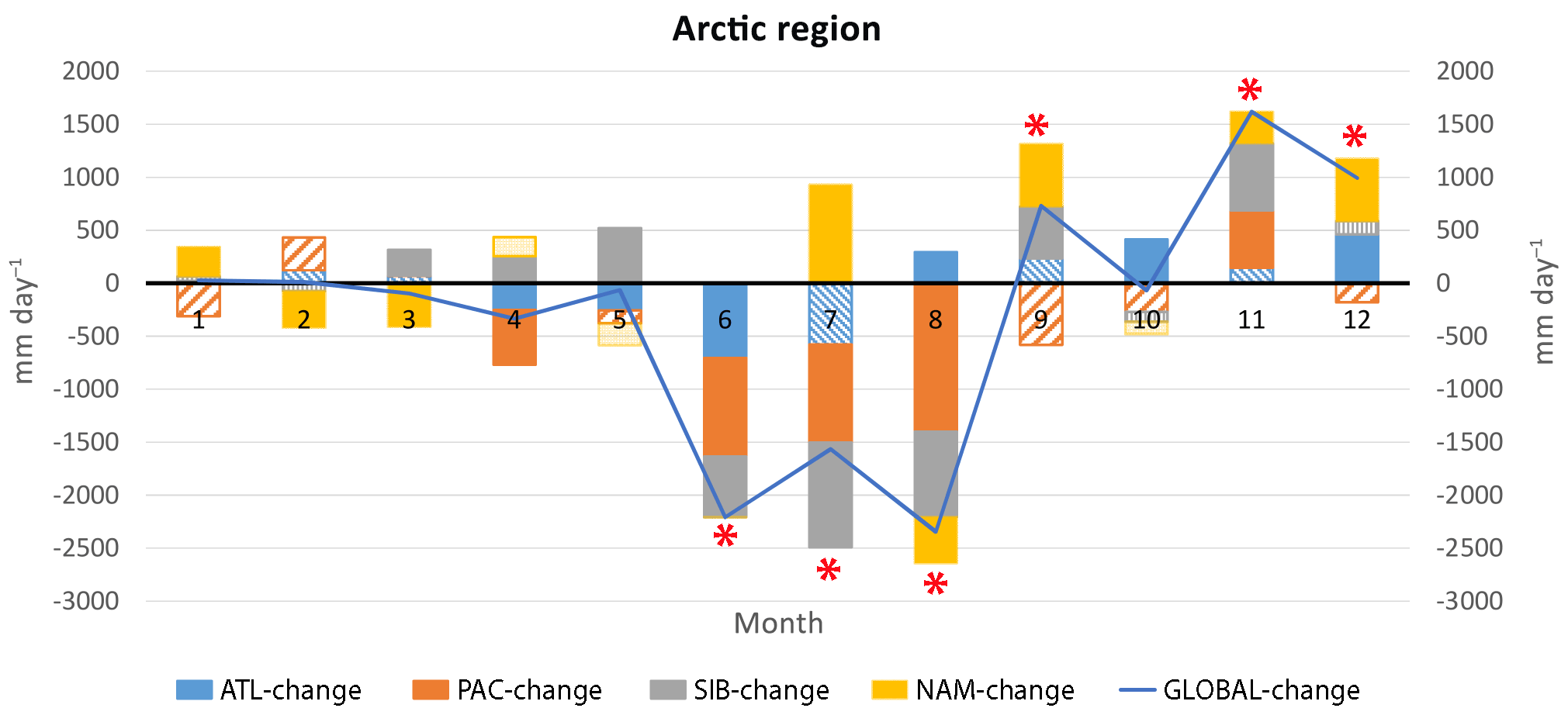
Figure 8Differences between mean values of moisture transport for precipitation (MTP) until 2003 and mean values after 2003 for every source region. Filled bars show those differences that are statistically significant at the 95 % confidence level for decreases after the CP. Statistical significance of the differences in total MTP (sum of the four sources) is displayed with a red asterisk.

Download

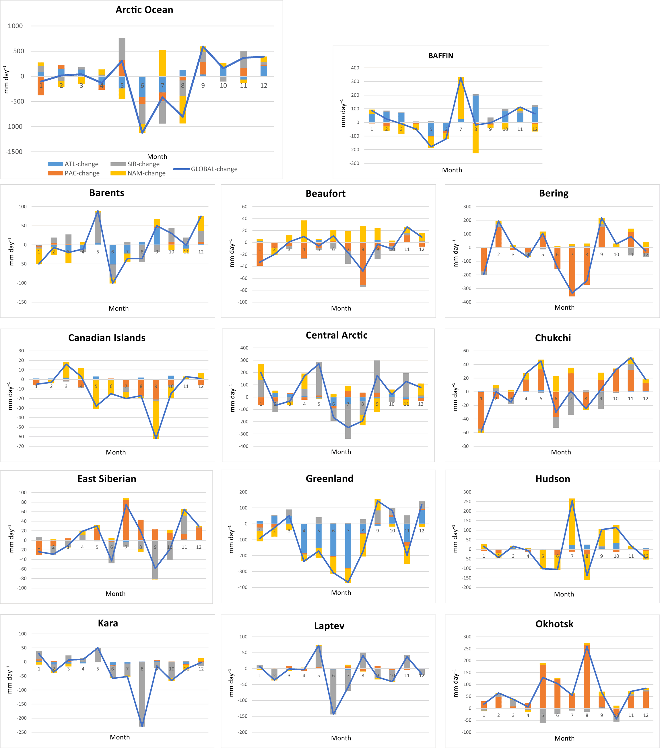
Figure 9Differences between mean values of moisture transport for precipitation (MTP) until 2003 and mean values after 2003 for every source region for the Arctic Ocean (AO) and its 13 subregions. Statistical significance of the differences is displayed in Table 1.

Download

Table 1Summary of the statistical significance of the MTP differences estimated by comparing daily values of moisture transport before and after the CP, based on the Student's t test. Circles indicate statistical significance at the 95 % confidence level for increases after the CP; crosses indicate statistical significance at the 95 % confidence level for decreases after the CP.

Download Print Version | Download XLSX

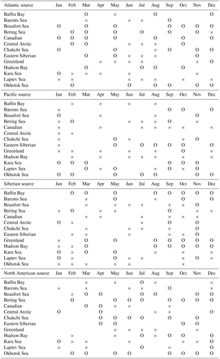
The analysis by subregion allowed us to identify which subregions contributed most to change in MTP in the AO. As in the case of the AR, the statistical significance of the differences (Table 1) has been estimated by comparing daily values of moisture transport before and after the CP. The diminished contribution of the Atlantic source to the AO in June and July is mainly attributed to the reduction of transport to Greenland; this decrease is not observed in August because of the compensation for the decrease to Greenland by the increase to Baffin Bay. A moderate increase in October and a small decrease in December were also attributed to changes occurring in Greenland. The slightly decreased contribution of the Pacific to the AO in summer was caused by the compensation for the decreased contribution of the Bering Sea (strong decrease) by a strong increase in the contribution of the Okhotsk Sea, with some influence of other regions such as the Beaufort Sea (decrease) and eastern Siberia (increase). There is greater concordance in autumn and winter, with generally slight increments, which resulted in a small increase in the contribution of the Pacific to the AO. The greatly decreased contribution of the Siberian source to the AO in summer is attributed mainly to the strong decrease in MTP to the central Arctic and Laptev Sea, and the generally slight increment of the contribution of the Siberian source for these regions in autumn and early winter (with the exception of October); these changes result in similar behaviour for the AO. The different changes of the contribution of the North American source to the AO in July (increase) and August (decrease) reproduce the common changes observed in the contributions to the Baffin and Hudson bays. The slight increase in contribution to the AO in September and October again is attributed to compensation for the increase to Hudson Bay by a strong decrease in September to the Canadian Arctic Archipelago and light decrease in October to Baffin Bay and the Barents Sea; the increased contribution of this source to the AO in December is the result of increased contribution to the central Arctic and the Barents Sea, partially compensated for by a slight decrease to the Hudson and Baffin bays.

3.3 Checking the Lagrangian results by analysing changes in vertical integrated moisture fluxes and atmospheric circulation patterns after and before Arctic sea ice change points

It is useful to check the results derived from the Lagrangian approach to estimate MTP with other Eulerian approaches such as the computation of vertical integrated moisture flux (VIMF). Supplement Fig. S1 shows the climatological VIMF by month in the period from June to December (left panel) and the difference between the periods after the CP and before the CP for the zonal component (central panel) and the meridional component of VIMF (right panel). This methodology cannot estimate specific changes in the MTP from each source to each sink as the more sophisticated Lagrangian approach does, but it is able to show whether patterns are compatible with the identified changes. For instance, in June (Fig. 10), the Atlantic source provides moisture for precipitation in the subregion of the Arctic Ocean named Greenland in our study, as revealed by the flux vectors in the top panel. However, the track of moisture from the source to the sink is clearly hindered for the period after the CP relative to the period before the CP, as revealed by negative values of the zonal component (blue colours in middle Fig. 10) in the band 45–60^∘ N latitude (less moisture transported from west to east, the direction of the source–receptor path) and negative values of meridional winds (blue colours in bottom Fig. 10) in the band 20–60^∘ W longitude (less moisture transported from south to north, the direction of the source–receptor path). We have carried out this analysis for each month, and for source and sink areas, and the patterns can explain all the significant results found in the Lagrangian analysis with almost absolute agreement (Fig. S1).

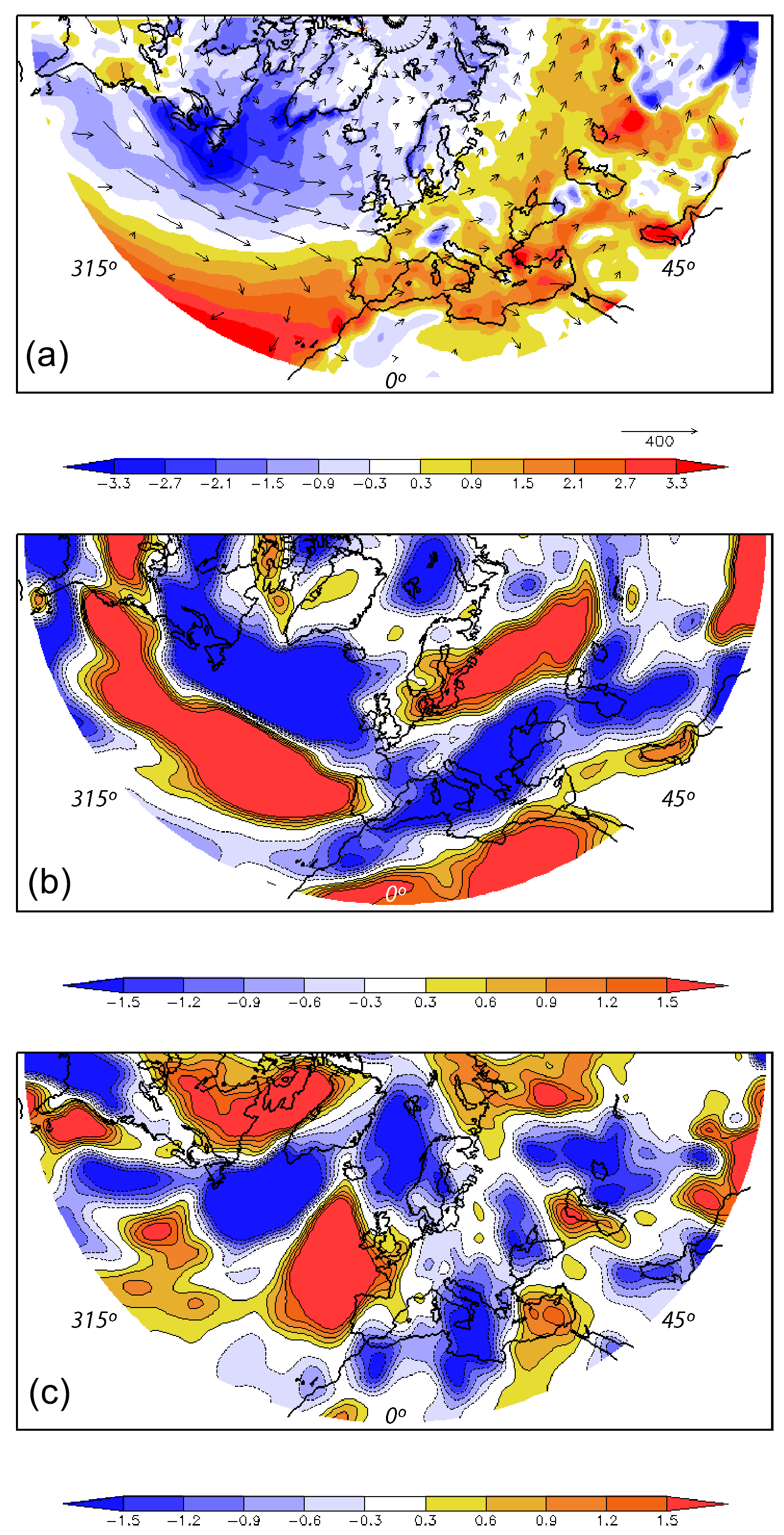
Figure 10(a) The climatological vertical integrated moisture flux (VIMF) (vector, kg m⁻¹ s⁻¹) and its divergence (shaded, mm yr⁻¹) in June for the European sector, (b) the difference between the periods after vs. before the CP for the zonal component of VIMF, and (c) as for panel (b) but for the meridional component of VIMF.

Download

An additional demonstration of the robustness of these results can be derived by analysing the changes in atmospheric circulation responsible for changes in moisture transport. Changes in MTP may be related to alterations in moisture sources caused by changes in circulation patterns, to changes in the intensity of the moisture sources because of enhanced evaporation, or to a combination of these two mechanisms. At a daily scale, changes in intensity are negligible, but changes in circulation may be significant. Thus, to analyse whether there are important differences in MTP from sources to sinks associated with different circulation patterns, and how such differences could affect MTP in the AR, we grouped individual days into four circulation types using the methodology developed by Fettweis et al. (2011) and explained in Sect. 2. We have separated the analysis into four sectors centred on the four sources of moisture to the AR to filter out annular effects, as we are interested in regional influences.

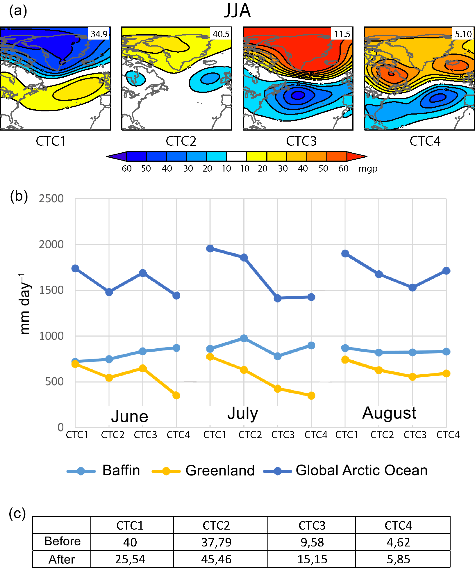
Figure 11(a) Anomalies of geopotential height at 850 hPa (Z850) for the four types of circulation centred in the Atlantic sector in summer (classes CTC1 to CTC4), and the percentages of days grouped in each class. (b) Average moisture transport for precipitation (MTP) for each class and summer months from the Atlantic source to the Arctic Ocean (AO), and the two dominant subregions, the Barents Sea and Greenland. (c) Change of frequency of these circulation types (classes) before and after the change point.

Download

Supplement Fig. S2 shows the summer and autumn types of circulation centred on the four source areas (Atlantic, Pacific, Siberia, and North America), with each individual map representing the anomalies of geopotential height at 850 hPa (Z850) for the four different classes found (from CTC1 to CTC4, with the percentage of days grouped). The average MTPs for each class before and after the CP are summarised in Table S2, whereas changes in the frequency of each class before and after the CP are shown in Table S3 (statistical significance changes were calculated using a z test to compare two sample proportions; Sprinthall, 2011). One of these sectors and one season can serve us as an example of these results: the Atlantic during summer (Fig. 11). The anomalies of geopotential height at 850 hPa (Z850) for the four different classes found (Fig. 11 top) show patterns that resemble the known teleconnection patterns in the region (Barnston and Livezey, 1987 and http://www.cpc.ncep.noaa.gov/data/teledoc/telecontents.shtml, last access: 18 December 2017). Thus, CTC1 has a zonal dipolar structure that resembles the positive phase of the eastern Atlantic pattern (a north–south dipole of anomaly centres that are positive in the southern one and span the North Atlantic); this pattern is closely related to enhanced precipitation on Greenland. CTC2 is slightly similar to the negative phase of the eastern Atlantic and western Russia (negative height anomalies located over Europe and northern China, and positive height anomalies located over the central North Atlantic and north of the Caspian Sea), associated with enhanced precipitation on the Barents Sea. CTC3 resembles the negative phase of the North Atlantic Oscillation (at above-normal heights across the high latitudes of the North Atlantic and below-normal heights over the central North Atlantic and western Europe), related to diminished precipitation on Greenland and enhanced precipitation on the Barents Sea. CTC4 is similar to the positive phase of the Scandinavian pattern (positive height anomalies over Scandinavia and western Russia) associated with diminished precipitation on the Barents Sea. Figure 11b shows the average MTP for each class in the summer months from the Atlantic source to the AO (dark blue line) and the two dominant subregions, the Barents Sea and Greenland (light blue and orange lines, respectively). CTC1 is the circulation type responsible for the highest MTP in the three summer months, and CTC3 and CTC4 are responsible for the lowest MTP, depending on the month. The change of frequency of these classes representing circulation types before and after the CP (Fig. 11 bottom) shows a decrease in the days belonging to CTC1, with the highest MTP from 40 to 25.4 days, and an increase in days belonging to CTC3 (from 9.58 to 15.15) and CTC4 (from 4.62 to 5.85), the two classes with the lowest MTP. These results are absolutely consistent with our Lagrangian results of changes in MTP. A similar analysis to the one for this sector, moisture source region, and season can be performed for all the significant results found in the Lagrangian analysis with very good agreement.