the Creative Commons Attribution 4.0 License.
the Creative Commons Attribution 4.0 License.
 | 09 May 2018
Changes in crop yields and their variability at different levels of global warming
Jacob Schewe
Katelin Childers
Katja Frieler
An assessment of climate change impacts at different levels of global warming is crucial to inform the policy discussion about mitigation targets, as well as for the economic evaluation of climate change impacts. Integrated assessment models often use global mean temperature change (ΔGMT) as a sole measure of climate change and, therefore, need to describe impacts as a function of ΔGMT. There is already a well-established framework for the scalability of regional temperature and precipitation changes with ΔGMT. It is less clear to what extent more complex biological or physiological impacts such as crop yield changes can also be described in terms of ΔGMT, even though such impacts may often be more directly relevant for human livelihoods than changes in the physical climate. Here we show that crop yield projections can indeed be described in terms of ΔGMT to a large extent, allowing for a fast estimation of crop yield changes for emissions scenarios not originally covered by climate and crop model projections. We use an ensemble of global gridded crop model simulations for the four major staple crops to show that the scenario dependence is a minor component of the overall variance of projected yield changes at different levels of ΔGMT. In contrast, the variance is dominated by the spread across crop models. Varying CO2 concentrations are shown to explain only a minor component of crop yield variability at different levels of global warming. In addition, we find that the variability in crop yields is expected to increase with increasing warming in many world regions. We provide, for each crop model, geographical patterns of mean yield changes that allow for a simplified description of yield changes under arbitrary pathways of global mean temperature and CO2 changes, without the need for additional climate and crop model simulations.
- Article
(4839 KB) -
Supplement
(458 KB) - BibTeX
- EndNote


Climate change exerts a substantial and direct impact on food security and hunger risk by altering the global patterns of precipitation and temperature which determine the location of arable land (Parry et al., 2005; Rosenzweig et al., 2014) as well as the quality (Müller et al., 2014) and quantity (Lobell et al., 2012; Müller and Robertson, 2014; van der Velde et al., 2012) of crops comprising most of the world food supply. By itself, climate change is expected to reduce global production of the four major crops wheat, maize, soy, and rice in current agricultural areas (Challinor and Wheeler, 2008; Peng et al., 2004; Rosenzweig et al., 2014). Facing an increasing food demand due to population growth and economic development, these reductions will have to be compensated for by (1) the direct physiological impacts of increased atmospheric CO2 concentrations (Kimball, 1983), which are beyond local human control; as well as (2) advances in agricultural management (e.g. fertilizer input or irrigation), technology, and breeding (Jaggard et al., 2010) or (3) expansion of agricultural land (Frieler et al., 2015; Smith et al., 2010).
In conjunction with these long-term changes, global warming is also expected to contribute to an increase in the frequency and duration of extreme temperatures and precipitation (droughts, floods, and heat waves), which may increase the near-term variability in crop yields and trigger short-term crop price fluctuations (Brown and Kshirsagar, 2015; Mendelsohn et al., 2007; Tadesse et al., 2014).
Anthropogenic emissions of greenhouse gases are expected to influence crop yields via several pathways. On the one hand, the associated climatic changes will modify the length of the growing season (Eyshi Rezaei et al., 2014), water availability, and heat stress (Lobell et al., 2012; Müller and Robertson, 2014; Schlenker and Roberts, 2009); and on the other hand, higher concentrations of atmospheric CO2 are expected to increase the water use efficiency in C3 (e.g. wheat, rice, soy) and C4 (maize) crops, and enhance the rate of photosynthesis in C3 crops (Darwin and Kennedy, 2000). Global gridded crop models (GGCMs) are particularly designed to account for these effects. They provide a complex process-based implementation of our current understanding of the mechanisms underlying crop growth, and are the primary tool for crop yield projections (Rosenzweig et al., 2014), which in turn are a prerequisite for assessing potential changes in prices (Nelson et al., 2014) and food security (Parry et al., 2005). However, these process-based crop yield projections rely on spatially explicit realizations of the driving weather variables such as temperature, precipitation, radiation, and humidity, often at daily resolution, as provided by computationally expensive global climate model (GCM) simulations. The GGCMs themselves also require significant computational capacity. These requirements generally limit the number and length of emissions scenarios that can be simulated.
The so-called pattern scaling approach is a well-established method to overcome these limits. Output from GCMs has been shown to be, to some extent, scalable to different global mean temperature (GMT) trajectories not originally covered by GCM simulations (Frieler et al., 2012; Giorgi, 2008; Heinke et al., 2013; IPCC-TGICA, 2007; Mitchell, 2003; Santer et al., 1990; Solomon et al., 2009). Scaled climate projections have also been used as input for different impact models (Ostberg et al., 2013; Stehfest et al., 2014) to achieve greater flexibility in terms of the range of emissions scenarios considered in climate impact studies.
Building upon such a framework, we present a method to extend the capacity of crop yield impact projections by relating simulated crop yield changes to two highly aggregated quantities – global mean temperature change (ΔGMT) and atmospheric CO2 concentration (pCO2) – by means of simplified function. ΔGMT and pCO2 are standard outputs of reduced-complexity climate models, which – while lacking the spatial resolution of complex GCMs – allow for highly efficient climate projections for any emissions scenario by emulating the response of the complex models (Meinshausen et al., 2011). Here “emulating” means that the simplified representation is designed to reproduce the global response of the complex model for the originally simulated scenarios but also allows for its inter- or extrapolation to other scenarios. We test to what extent crop yield changes, as one example of climate change impacts, can be described directly in terms of GMT and pCO2 changes. Our approach is different from other emulators which use spatially explicit climate projections as input for the simplified functions (Blanc, 2017; Oyebamiji et al., 2015). While these approaches only emulate the responses of the complex crop model, the approach presented here implicitly provides a simplified description of both the GCMs' regional patterns of climate change and the associated response of the crop models. Such an approach provides high computational efficiency, making it applicable, for example, in integrated assessment models. In principle, other emulators could be used in this setting; however, they require an additional step of first scaling the climatic changes to the specific emissions scenario.
The emulator introduced here allows for multi-crop-model projections for arbitrary emissions scenarios as long as crop-model ensemble projections are available for a limited set of scenarios. This offers a practical way of keeping track of a relevant but often-ignored source of uncertainty which is manifested in the considerable spread across different crop models and other process-based impact models (Rosenzweig et al., 2014; Schewe et al., 2014). This uncertainty is particularly critical when estimating socio-economic consequences (Nelson et al., 2014).
We test the approach using an ensemble of yield projections of the four major crops maize, rice, soy, and wheat, generated within the first phase (“Fast Track”) of the Inter-sectoral Impact Model Intercomparison Project (Warszawski et al., 2014). For a number of ΔGMT intervals we compare the spread in yield outcomes induced by the choice of emissions scenario with that induced by the choice of GGCM and GCM. A low scenario-induced spread means that GCM- and GGCM-specific yield projections can be approximated by a simplified relationship with GMT change without accounting for the underlying emissions scenario, which is a prerequisite to applying the simplified relationship to other emissions scenarios. The test is performed at each grid point and separately for simulations of purely rain-fed yields and fully irrigated yields. Multi-model ensembles in the ISIMIP data archive provide a uniquely broad suite of crop yield simulations over a wide range of crops, CO2 concentrations, and irrigation options encompassing output from five GGCMs, forced with output from up to five GCMs under four Representative Concentration Pathways (van Vuuren et al., 2011).
In Sect. 2 we describe the ISIMIP data and the methods used to test for scenario dependence and adjustment for different levels of pCO2. Section 3 is dedicated to the presentation of the projected average changes in crop yields at different levels of global warming and an attribution of the variance of these long-term changes to different sources of uncertainty, i.e. different GCMs, different GGCMs, and different emissions scenarios (Sect. 3.1). In addition, we test to what degree the scenario dependence of crop yields at a specific level of global warming can be explained by different levels of pCO2 (Sect. 3.2). Finally, we provide individual maps of yield changes at different levels of GMT and the additional effect of variations in pCO2 at the respective GMT levels. We propose three methods to generate these patterns based on the available complex model simulations, and describe the related approaches to estimate GGCM- and GCM-specific yield changes for new ΔGMT trajectories not originally covered by GCM–crop-model simulations. In Sect. 4 we present a quantification of the projection errors compared to actual simulations by the complex gridded crop models. Finally, in Sect. 5 we quantify the residual inter-annual variance of the simulated crop yields in terms of GMT change across all combinations of crop and climate models. Section 6 provides a summary.
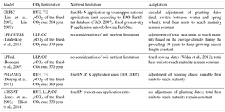
(Liu, 2009; Liu et al., 2007)(FAO, 2007)(Lindeskog et al., 2013)(Bondeau et al., 2007)(Waha et al., 2012)(Deryng et al., 2011)(IFA, 2002)(Elliott et al., 2014; Jones et al., 2003)Table 1Basic crop model characteristics with respect to (1) the implementation of CO2 fertilization effect – as affecting radiation use efficiency (RUE), transpiration efficiency (TE), leaf-level photosynthesis (LLP), or canopy conductance (CC); (2) accounting for nutrient constraints and associated assumption with respect to fertilizer application (N: nitrogen; P: phosphorus; K: potassium); (3) implemented adaptation measures.
2.1 Crop yield simulations
We use projections from five different GGCMs (GEPIC, LPJ-GUESS, LPJmL, PEGASUS, and pDSSAT) that participated in the first phase of ISIMIP (Rosenzweig et al., 2014; Warszawski et al., 2014) in order to test for a dependence of projected yield changes on the GMT pathway (see Sect. 1 for their basic characteristics). Each crop model was forced by climate projections from five different GCMs (HadGEM2-ES, IPSL-CM5A-LR, MIROC-ESM-CHEM, GFDL-ESM2M, NorESM1-M) generated for four RCPs (RCP2.6, RCP4.5, RCP6.0, RCP8.5) in the context of the Coupled Model Intercomparison Project, phase 5 (Taylor et al., 2012). CMIP5 was an effort by the climate modelling community to provide a new suite of climate simulations in time for the Intergovernmental Panel on Climate Change (IPCC) Fifth Assessment Report (AR5). The RCPs cover the range from climate mitigation (RCP2.6, RCP4.5) to business-as-usual (RCP6.0) and high-emissions scenarios (RCP8.5). Climate projections have been bias corrected to better match observed historical averages of the considered climate variables. For the future, the bias-correction preserves absolute changes in monthly temperature and relative changes in monthly values of the other variables simulated by the GCMs while also correcting the daily variability about the monthly mean (Hempel et al., 2013). Separate simulations are available for each of the four major crops, wheat, maize, rice, and soy, on a global 0.5 ∘ × 0.5∘ grid, covering the time period from 1971 to 2099. The considered crop is assumed to grow everywhere on the global land area, only restricted by soil characteristics and climate but independent of present or future land use patterns (“pure crop” simulations). Each model has provided a pair of simulations (“runs”) for each climate change scenario: (1) a rain-fed run and (2) a full-irrigation run assuming no water constraints. This design provides full flexibility with regard to the application of future land use and irrigation patterns. While the crop yield () in “default” simulations accounts for the fertilization effects due to the increasing levels of pCO2, the ISIMIP setting also includes a sensitivity experiment in which the crop models were forced by the same climate change projections but pCO2 was kept fixed at a “present-day” reference level that differs from GGCM to GGCM (see Table 1). We will refer to this run as the “fixed-CO2” run and indicate the associated crop yields by . As a special case, the default simulations for pDSSAT do not use annual pCO2 changes. Instead, pCO2 was changed every 30 years using the average pCO2 of the respective 30-year time slice.
2.2 Effect of temperature change
We analyse the dependence of yield changes on ΔGMT separately for rain-fed and full-irrigation simulations, and for each crop. While yields in a given grid cell of course depend on the local temperature, long-term changes in local temperature are in turn a manifestation of global greenhouse-gas related warming (Frieler et al., 2012). The aim here is testing to what extent local long-term changes in yields can be described in terms of a single global measure of warming, ΔGMT. Since the time of attaining a given ΔGMT differs between GCMs and scenarios, we group all available data into ΔGMT intervals (bins) separated by 0.5 ∘C steps with 0.5 ∘C width (±0.25 ∘C around the central temperature), where ΔGMT is calculated relative to the present-day (1980–2010 average) reference level. For all annual data falling into a given interval and at each grid point we apply a separate one-way analysis of variance (ANOVA fixed-effects model) to individually calculate the yield variance explained by (1) different GGCMs, (2) the GCMs, and (3) the RCPs. The quantification of the RCP dependence of the relationship between global warming and yield change is limited to warming levels of up to 2 to 3 ∘C above present depending on the GCM because only one RCP (RCP8.5) reaches temperatures above this threshold. However, we also provide the patterns of yield change for the higher concentration scenario. In the main text, all figures except Figs. 9 and 10 refer to a ΔGMT level of 2.5 ∘C, and all figures except Figs. 3, 4, and 11 refer to crop model simulations driven by HadGEM2-ES climate. See Fig. 1 for the years associated with ΔGMT = 2.5 ∘C in HadGEM2-ES. The Supplement (Ostberg et al., 2018) contains analogous figures for other GMT levels and GCMs.
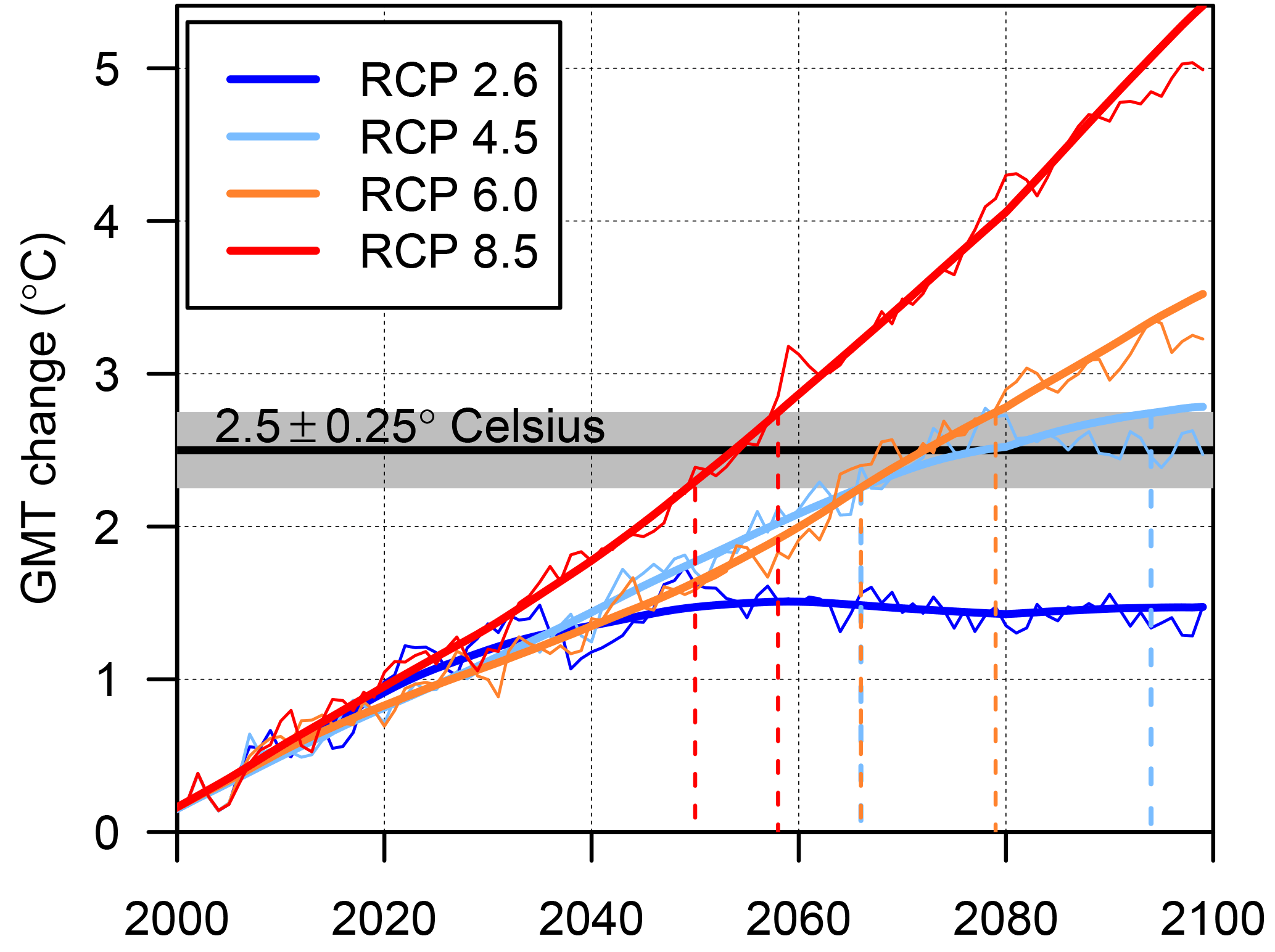
Figure 1GMT projections from HadGEM2-ES for the four RCPs. The horizontal line and shading indicate the 2.5 ∘C bin. The original annual GMT values (thin lines) are smoothed (thick lines) in order to obtain a contiguous time interval for each ΔGMT bin. The smoothing is based on a singular spectrum analysis with a time window of 20 years (Golyandina and Korobeynikov, 2014; Golyandina et al., 2015; Korobeynikov, 2010). Years where the thick line falls within the shaded area are associated with ΔGMT = 2.5 ∘C, and the corresponding time interval is delineated by the dashed vertical lines.
We do not impose a specific functional relationship between GMT change and change in crop yields. Yield change for any GMT level between the central levels of the considered bins could be derived by a simple linear interpolation among the patterns of neighbouring bins but without assuming a linear relationship between global mean warming and yield change across the full range of warming.
2.3 Effect of pCO2 change
The direct effect of CO2 fertilization on crop yields is expected to introduce some scenario dependence into the relationship between GMT change and yield change. We test to what degree the scenario dependence of the relationship can be explained by introducing pCO2 as an additional predictor for within-bin fluctuation of yields. To this end, we evaluate two different approaches to estimate the direct CO2 effect on crop yields within the different GMT bins, described in detail below. The two approaches differ in terms of the crop model simulations that they require: approach (a) only requires the default crop yield simulations with increasing pCO2 whereas approach (b) requires a pair of simulations with increasing pCO2 and with fixed pCO2 at the present-day reference level.
2.3.1 Approach (a)
For all years falling into a specific ΔGMT bin, approach (a) fits the following linear regression model to the response of yields in the default simulation to the increase in pCO2:
where , t) is the absolute yield change in grid point i and year t with respect to the historical reference period (1980–2010) and pCO2(t) is the atmospheric CO2 concentration of the corresponding year. In this statistical model, two parameters are determined by regression: ΔYclim(i) represents an estimate of the purely climate-induced yield change at the respective bin temperature, but assuming a fixed year-2000 pCO2 of 370 ppm (i.e. without CO2 fertilization), and a1(i) represents the added effect of CO2 fertilization. Finally, ϵ(i, t) ∽ N(0, σ2) represents the residual error.
2.3.2 Approach (b)
Approach (b) fits the following linear regression model to the yield difference between the default and fixed-CO2 simulation for all years falling into a specific ΔGMT bin:
where , t) and , t) is the absolute yield in grid point i and year t of the default and fixed-CO2 simulations, respectively; pCO2(t) is the atmospheric CO2 concentration of the default simulation during the respective year; and pCO is the crop-model-specific pCO2 value of the fixed-CO2 simulation (see Table 1). In this statistical model, a1(i) is determined by regression and represents the CO2 fertilization effect, and ϵ(i, t) ∽ N(0, σ2) represents the residual error. No intercept is estimated in this model because yields from the default and fixed-CO2 runs are expected to be identical if pCO2(t) = pCO. The purely climate-induced yield change at a fixed year-2000 pCO2 of 370 ppm ΔYclim(i) can then be derived as
where is the average yield change in the respective warming bin of the fixed CO2 simulation with respect to the historical reference period and a1(i) ⋅ (pCO − 370 ppm) corrects for the different pCO used by each GGCM.
2.4 Emulator of temperature and CO2 effects
Based on the spatial patterns of purely climate-induced yield change ΔYclim(i) and added CO2 fertilization effect a1(i), which are derived separately for each rain-fed and irrigated crop and specific to each crop model and GCM, we propose the following two-step interpolation method to compute crop yield changes for any given pair of ΔGMT and pCO2, using either the coefficients from approach (a) or (b):
-
linear interpolation of ΔYclim(i) between the two neighbouring ΔGMT bins to the desired ΔGMT value;
-
addition of the CO2 pattern described by a1(i) ⋅ (pCO2 − 370 ppm), where a1(i) is also interpolated linearly between the respective coefficients from the neighbouring ΔGMT bins.
The application of these two steps using coefficients from method (a) above will be called emulator approach (a); their application using coefficients from regression method (b) will be called emulator approach (b). In addition, we propose a third, very basic emulator approach (c) in which the yield change for any given ΔGMT is derived from a simple linear interpolation of the average yield change in the neighbouring warming bins of the default simulations with respect to the historical reference period, without using the associated pCO2 as an additional predictor.
The linear interpolation of any of the previous coefficients between two neighbouring warming bins is illustrated for a ΔGMT of 2.3 ∘C as follows:
where coef can be ΔYclim(i), a1(i), or .
Using GGCM projections for the HadGEM2-ES climate input to train the emulators, we test which of the emulator approaches, (a), (b), or (c), provides the best reproducibility for yield changes simulated under the four RCPs (Sect. 4). While approach (b) requires a pair of crop model simulations – one with time-varying pCO2 and one with fixed present-day pCO2 – approaches (a) and (c) only require the default simulations with time-varying pCO2. Thus, a comparison of the three approaches could provide some important guidance regarding future crop model experiments required to allow for the proposed highly efficient emulation of crop model simulations. Since simulated crop yields are subject to considerable inter-annual variability, we also test what effect the number of available training data has on the reliability of the derived regression coefficients. For that purpose, we train the emulators using either all available simulation data from the four RCPs or only simulation data from RCP8.5 and compare the fraction of the land surface for which derived fits are statistically significant as well as the difference between simulated and emulated yield changes. Due to the 30-year time slices of constant pCO2 used by pDSSAT in the default run, approach (a) cannot be applied to this model using only RCP8.5 data. Since only RCP8.5 reaches ΔGMT > 3.5 ∘C, this limits the temperature range of emulator approach (a) for pDSSAT even when using all available training data.
We evaluate and compare the performance of the three emulator approaches at the grid scale as well as the scale of large regions. Grid point yields (in tons per hectare) are multiplied by the fixed year-2000 crop-specific growing area from the MIRCA2000 dataset (Portmann et al., 2010) to derive regional total crop production (in tons). MIRCA2000 provides gridded growing areas for a total of 26 rain-fed and irrigated crops based on a combination of census, remote sensing, and other geographic data sources.
3.1 Patterns of relative changes at different levels of global warming and main sources of variance
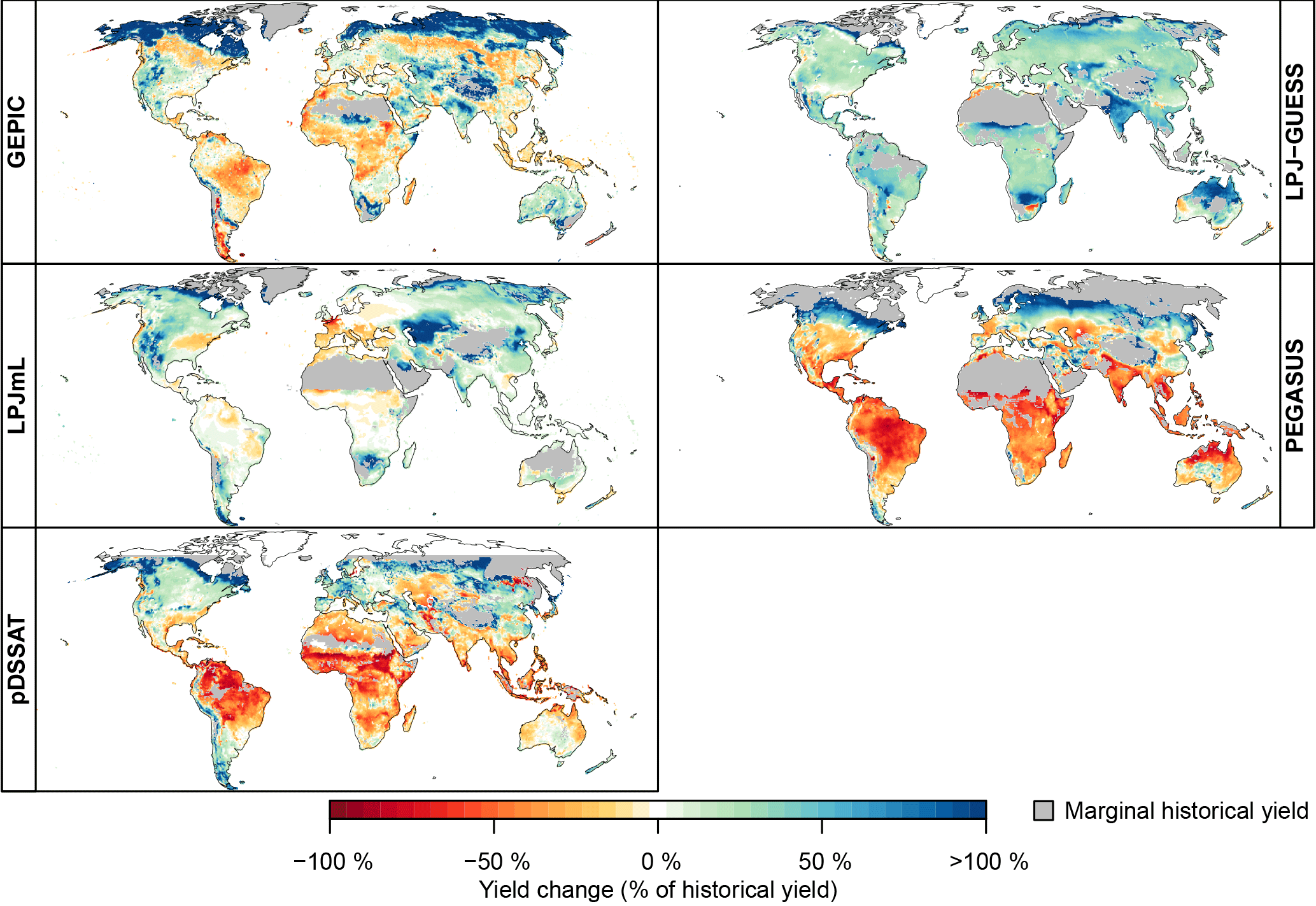
Figure 2Average wheat yield change at ΔGMT = 2.5 ∘C as a percentage of the mean historical yield (1980–2010 average) under rain-fed conditions for each crop model forced by HadGEM2-ES. The average is calculated across all RCPs which reach the global mean warming interval from 2.25 to 2.75 ∘C, namely RCP4.5, RCP6.0, and RCP8.5. Note that pDSSAT is run over a limited domain excluding areas north of 60∘ N. Regions with marginal historical yields (defined as lying below the 2.5 % quantile of historical yields on year-2000 cropland) are masked to avoid exaggerated relative yield increases. Analogous figures for different crops, for irrigated conditions, and for absolute yield change (in tons per hectare) are available in the Supplement.
In general, increasing GMTs correspond to an expansion of arable land to higher latitudes with concurrent yield reductions in equatorial regions. The highest positive changes in projected yields under rain-fed conditions at 2.5 ∘C ΔGMT are typically in the northern high latitudes and mountainous regions for all crops (Fig. 2 for wheat; figures for other crops in the Supplement). These locations were previously inhibited by a short growing season, which extends with increasing air temperature (Ramankutty et al., 2002). Yield gains also occur over previously moisture-limited regions, such as the northwestern US and northeastern China, in agreement with the findings of Ramankutty et al. (2002). In contrast, near the Equator most crop yields decrease, especially maize and wheat. Since most cultivated land currently lies in low and middle latitudes, potential yield changes in those regions contribute a higher relative importance for today's food production system than changes in high latitudes.
While variations exist in the magnitude of projected yield changes, there is a high degree of consistency in the direction of yield change across ensemble members, especially over the high latitudes, where most of the largest projected yield changes occur, but where yields are in general smaller (Fig. 3). Utilizing output from all available combinations of GCM, GGCM, and RCP scenarios, more than three-quarters of the ensemble members indicate increasing crop yields over the upper mid-latitudes in the Northern Hemisphere for all crops at 2.5 ∘C.
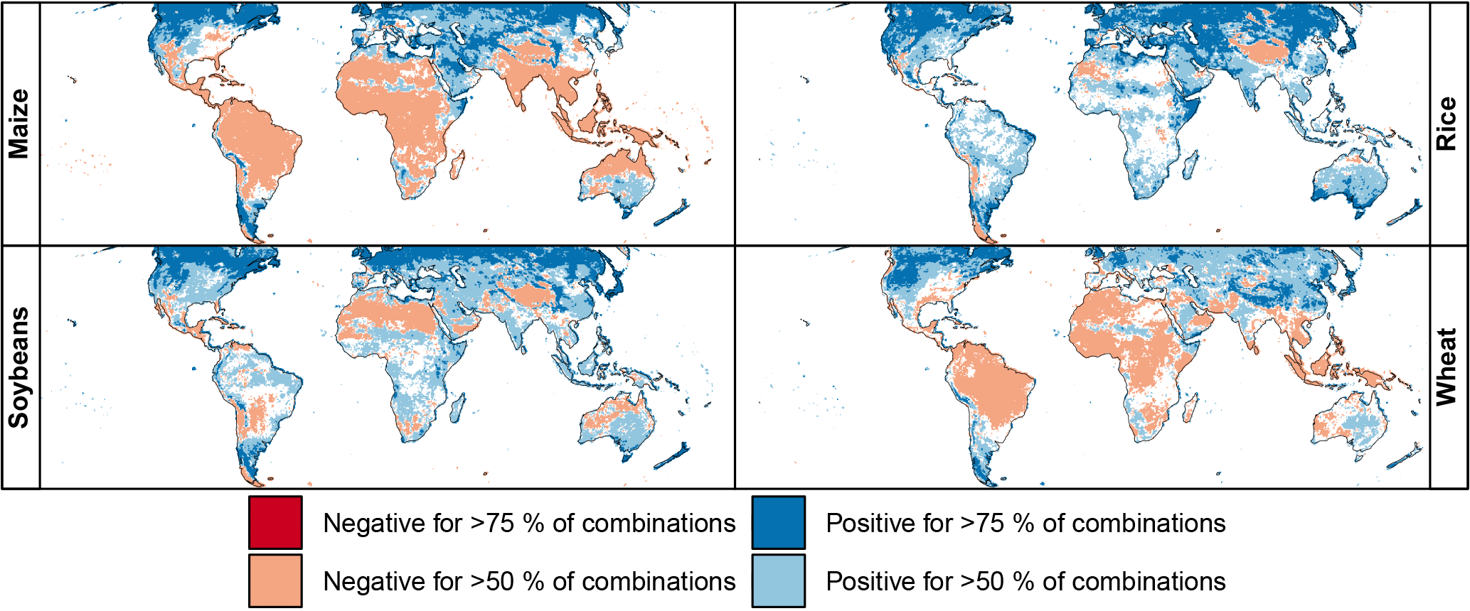
Figure 3Percentage of crop model simulations (combination of a single GCM, GGCM, and RCP scenario) indicating an increase (blue) or decrease (red) in yield of greater than 5 % at each grid point at 2.5 ± 0.25 ∘C ΔGMT as compared to the historical period for maize, rice, soybeans, and wheat under rain-fed conditions. White indicates either a change of less than 5 % or disagreement among the models in the direction of yield change. Note that only four out of five GGCMs provided results for rice. An analogous figure for irrigated conditions is available in the Supplement.
The simulated yield values at each grid point and within each GMT bin are subject to variation due to the selection of impact model, GCM forcing, and emissions scenario. When considering all of these factors, the variance attributable to the impact model selection is much greater than that associated with the GCM or scenario choice in most regions (Fig. 4). This holds for rain-fed as well as irrigated simulations. The predominance of the impact model component in total variance is particularly evident in the middle to high latitudes for all four considered crops, where impact model variance accounts for up to 90 % of the grid point variance at 2.5 ∘C.
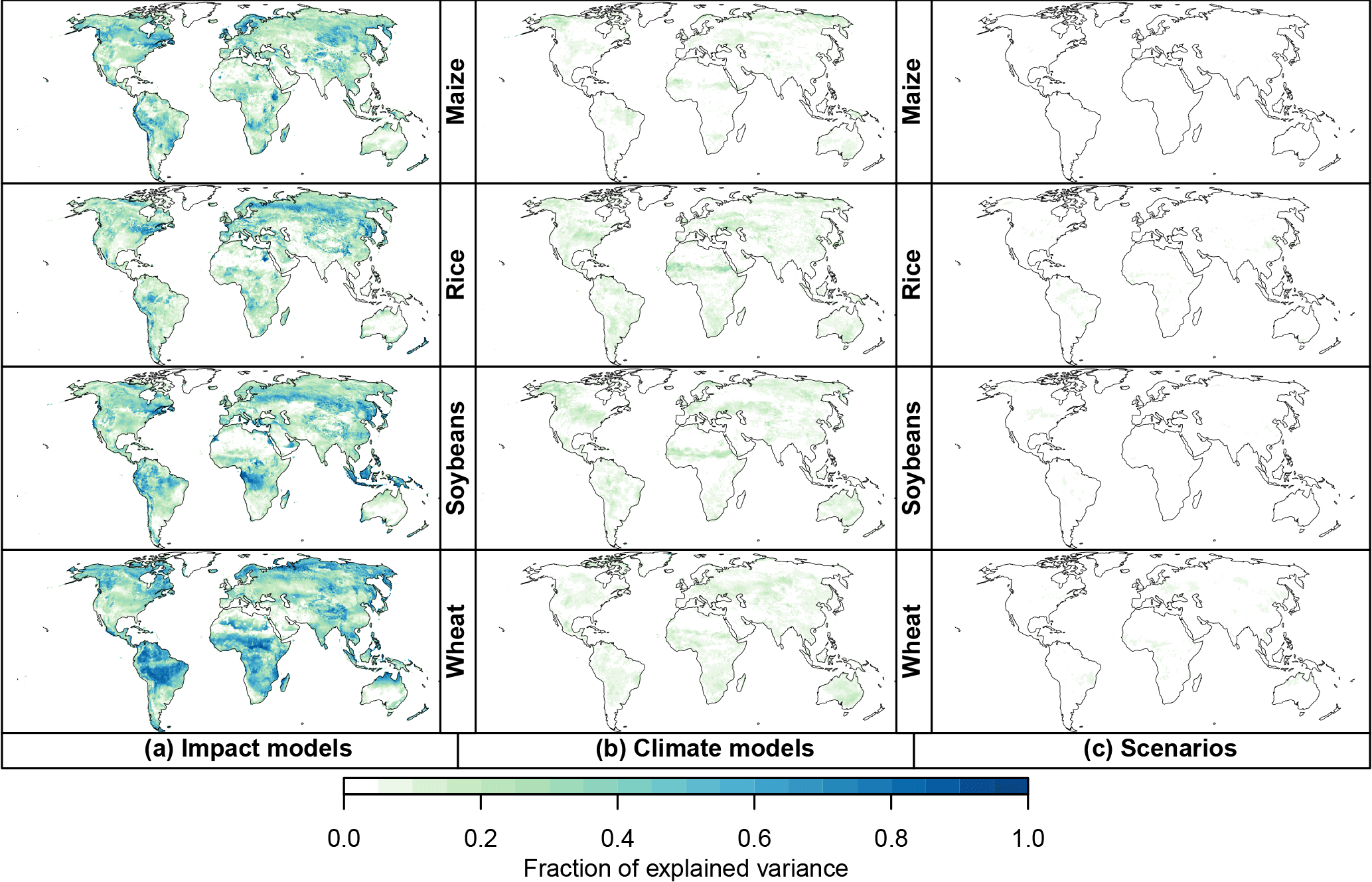
Figure 4Fraction of total yield variance attributable to the impact models (GGCMs, a), climate models (GCMs, b), and scenarios (RCPs, c) for each crop. Figure shown for rain-fed runs at ΔGMT = 2.5 ± 0.25 ∘C warming; an analogous figure for irrigated runs is provided in the Supplement.

Figure 5Difference in global mean yield change (sum of rain-fed and irrigated, and weighted by year-2000 growing areas) between the default () and fixed-CO2 simulations (), for each crop over the range of pCO2 associated with the ΔGMT = 2.5 ∘C bin. Results are as simulated by LPJmL forced with output from HadGEM2-ES. Each colour represents an emissions scenario. Points mark individual years while dotted lines and shaded areas indicate the linear best fit and its 95 % confidence interval for each scenario. The black dotted line indicates the linear best fit through all available scenarios. Analogous figures for other GGCMs and warming bins are available in the Supplement.
3.2 Direct impacts of increasing pCO2
In addition to air temperature warming, pCO2 has a direct influence on crop yields. As it varies within the different ΔGMT bins, it is expected to induce part of the fluctuations of the yield changes at given GMT levels. We find that this CO2 effect shows little scenario dependence (see Fig. 5 for the global average effect within the LPJmL simulations at ΔGMT = 2.5 ∘C), consistent with a short response time of plants to pCO2 changes. As expected, the CO2-induced yield differences increase with heightened atmospheric CO2 level under all emissions scenarios, implying a stronger CO2 fertilization impact with increased pCO2.
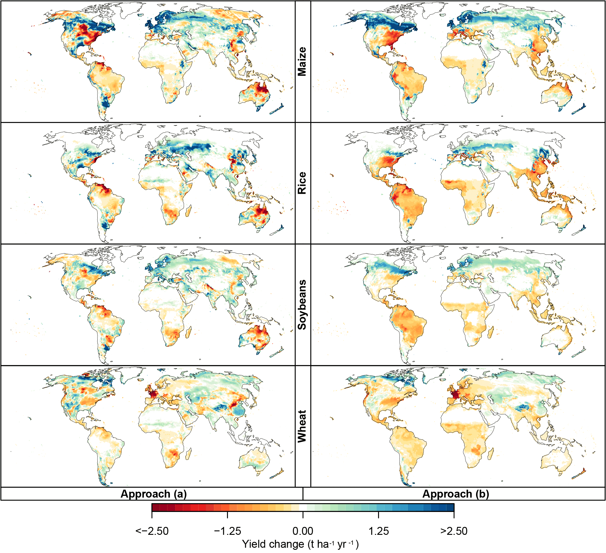
Figure 6Climate-change-induced yield changes at ΔGMT = 2.5 ∘C of global warming and the year-2000 pCO2 level (370 ppm). Left column panels: patterns of ΔYclim(i) derived at each grid point i using approach (a) (see Eq. 1). Right column panels: corresponding patterns of ΔYclim(i), derived using approach (b) (see Eq. 3). Both types of patterns are derived from LPJmL simulations forced by HadGEM2-ES assuming rain-fed conditions and expressed as absolute differences compared to the historical period (1980–2010). Rows: different crop types. Analogous figures for irrigated conditions, for different GGCMs, and using relative instead of absolute yield changes are available in the Supplement.

Figure 7CO2-induced yield changes at 2.5 ∘C of global warming for LPJmL forced by HadGEM2-ES assuming rain-fed conditions. Analogous to Fig. 6, but showing the scaling coefficients a1(i) from approach (a) (left column panels) and approach (b) (right column panels), multiplied by the average pCO2 change compared to the year 2000 (370 ppm) across all years falling into the GMT bin. Rows: different crop types. Analogous figures for irrigated conditions, for different GGCMs, and using relative instead of absolute yield changes are available in the Supplement.
At the grid point level, two approaches have been used to separate purely climate-change-induced from CO2-induced yield change (following Eqs. 1 to 3). Figure 6 shows the climate-change-induced yield change at ΔGMT = 2.5 ∘C for LPJmL under rain-fed conditions, using all available runs that fall into the warming bin to estimate ΔYclim(i). Figures for irrigated conditions and the other GGCMs are available in the Supplement. The two methods result in broadly similar patterns, with yield increases in the upper middle and high latitudes, mixed regions with decreases and increases in the lower mid-latitudes, and mostly decreases in the tropics. However, the magnitude of change differs between the two approaches: approach (a) generally estimates larger changes outside the tropics while yield decreases in the tropics are larger in approach (b). There are also some regions where both approaches disagree regarding the direction of change, such as the high latitudes of both western North America and eastern Russia for wheat and parts of Southeast and South Asia for all crops. Patterns of climate-induced yield change match better between both approaches under irrigated conditions (see Supplement).
In GEPIC, both approaches disagree on the direction of change for maize yields over large parts of Europe. In LPJ-GUESS, both approaches disagree on the direction of change in most of the tropics for all crops. While tropical yield change is predominantly negative in approach (b) mirroring results of the other crop models, approach (a) estimates mostly positive climate effects on tropical crops. In pDSSAT, approach (a) generally produces larger areas with negative yield change than approach (b). At the same time, positive yield effects in approach (a) have a larger magnitude than those in approach (b) in many regions. In PEGASUS, both approaches disagree on the direction of change over large parts of the US for maize and soybeans, and large parts of China for wheat.
The estimates of CO2-induced yield change also differ between the two approaches (Fig. 7 for LPJmL results under rain-fed conditions). We expect CO2 fertilization to have a positive or at least neutral effect on yields, and this is confirmed by approach (b) for all GGCMs and crops. Only GEPIC simulations show negative CO2 effects on soybean and wheat yields in a few regions for approach (b). This can be explained by nutrient interactions in the model: CO2 fertilization leads to yield increases first but also increases nutrient depletion in the soil compared to the fixed-CO2 run. If fertilizer application is insufficient to replenish nutrient stocks this can lead to lower yields despite the beneficial effect of higher pCO2. With approach (a), however, areas of negative estimated CO2 effects are widespread in all GGCMs and all crops. Generally, the magnitudes of the estimated CO2 effect are also much larger, often surpassing those of approach (b) even in regions where the direction of change matches.
Given that approach (a) contradicts our expectation of how CO2 fertilization should affect yields in many regions, we conclude that approach (a) is not reliable in separating the effects of climate change on yield from those of pCO2 change. By design, climate-induced and CO2-induced yield changes add up to the full yield change (see Eq. 1), which is why the difference among the patterns of estimated CO2 effects explains why climate change patterns from Fig. 6 also differ substantially between both approaches in some regions. Approach (a) has a structural disadvantage to approach (b) in that it estimates both the climate-induced and CO2-induced effect on yields from the same linear regression model (Eq. 1). In addition to changes in pCO2 annual yields in each warming bin are subject to substantial inter-annual climate variability, which means that individual years with a higher pCO2 do not necessarily have a higher yield. In contrast, approach (b) only estimates the CO2-induced yield change from the regression model (Eq. 2) while both the default and the fixed-CO2 runs are subject to identical climate variability. There is inter-annual variability in the CO2-induced yield change as well (see Fig. 5 for the global average effect); however, it is much smaller than the total yield variability.
While approaches (a) and (b) should provide similar estimates of the CO2-induced yield change given a large sample, our sample size is limited by the number of years falling into each ΔGMT bin (Table 2). This number varies between 7 years in the 4.5 and 5.0 ∘C bin and up to 66 years in the 1.0∘C bin when yield data from all RCPs are used to train the emulator. The number of years varies between 7 and 13 years if only data from RCP8.5 are used. Given the limited sample size and possibly large variability, the derived fits are often not statistically significant. For approach (a) we found that derived fits were rarely significant on more than 25 % of the crop-specific growing area (Portmann et al., 2010) using a p value of 0.05 (figure available in the Supplement). Values were even lower if only RCP8.5 was used for the regression. In contrast, fits derived using approach (b) were mostly statistically significant (p < 0.05) on more than 70 % of the growing area, often on more than 90 % of the area. We also found only a small negative effect in terms of statistical significance if only RCP8.5 was used in approach (b).
Table 2Number of years of yield data available in each ΔGMT bin for HadGEM2-ES. Only RCP8.5 reaches warming levels above 3 ∘C.
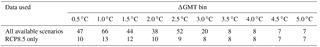
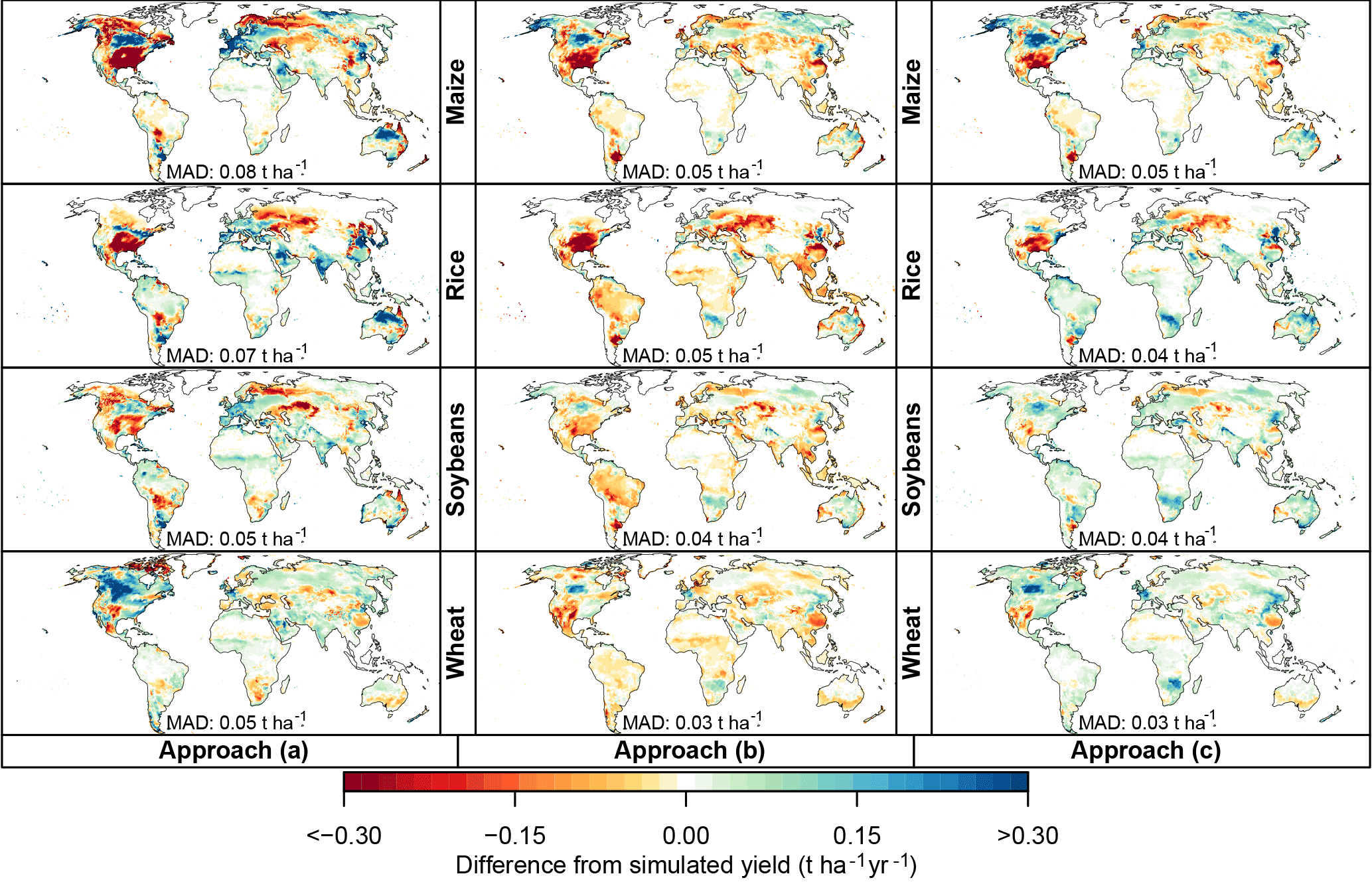
Figure 8Validation of the three emulator approaches. Maps show the difference (emulated minus simulated) among the simulated LPJmL yields forced by HadGEM2-ES climate for RCP4.5 under rain-fed conditions, averaged over all years falling into the ΔGMT bin of 2.5 ∘C (2066–2094), and the emulated yields for the same years based on approach (a) (left column panels), approach (b) (middle column panels), and approach (c) (right column panels). Rows: different crops. MAD: mean absolute difference, regardless of sign, averaged across all grid points. Analogous figures for irrigated conditions and for different GGCMs are available in the Supplement.
Using GGCM projections for the HadGEM2-ES climate input, we test which of the approaches, (a), (b), or (c), provides the best reproducibility for all four RCPs. For that purpose, we apply each emulator with a time series of ΔGMT and pCO2 from the RCPs and compare emulated yield changes in each grid point as well as total crop production for 10 large world regions to those simulated by the GGCM. For pDSSAT, the pCO2 time series used in that model's default run is also used with the emulator.
Figure 8 shows results for the LPJmL model, when applying the emulators trained on all available data to reproduce rain-fed yields under RCP4.5. Figures for other RCPs, irrigated yields, and other GGCMs are available in the Supplement.
Approach (a) generally leads to the largest differences relative to the simulated yield change (Fig. 8, left column). In particular maize, rice, and soybean yields are underestimated for much of North America, and overestimated in Europe, temperate South America, and Australia. Wheat yields are overestimated in Canada, for example.
Approach (b) also leads to some substantial deviations from the yields simulated by LPJmL, mainly in the Northern Hemisphere (Fig. 8, middle column). Spatial patterns of over- and underestimation are broadly similar to approach (a), but the magnitude of the difference is generally slightly lower. In the tropics, approach (b) often leads to a higher deviation from the simulated yields than approach (a), particularly for rice and soybeans in South America.
Finally, approach (c) leads to a similar pattern of deviations from the simulated yields as approach (b) for maize (Fig. 8, right column). For the other crops, approach (c) often leads to an overestimation of yields whereas approach (b) tends to underestimate simulated yields. The mean absolute deviation between emulated and simulated yields (designated as MAD in Fig. 8) is similar for approaches (b) and (c). Approach (c) performs slightly better than approach (b) for rice, and both approach (b) and (c) perform better than approach (a) for all four crops. Differences among the three emulators are smaller when reproducing RCP6.0 and RCP8.5 (figures available in the Supplement).
Table 3Root-mean-square difference between emulated and simulated decadal production (expressed as a percentage of the simulated production as in Fig. 9) in the largest producing region of each crop, for all five crop models forced by HadGEM2-ES climate projections. Average across all four RCPs. The values for all combinations of models, crops, and regions, and separately for each RCP, can be found in the Supplement. Top: emulators trained on all available data; bottom: emulators trained on RCP8.5 only.
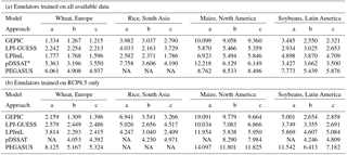
* Emulator approach (a) for pDSSAT only covers warming of up to 3.5 ∘C, i.e. up to 2070 under RCP8.5. NA: not available.
The difference between emulator approaches (b) and (c) is even smaller in the other crop models than in LPJmL (figures available in the Supplement). Overall, MAD between emulated and simulated yields is up to 50 % higher than LPJmL in PEGASUS, roughly twice as high in GEPIC, and up to 3 times as high in pDSSAT. In LPJ-GUESS, MAD between emulated and simulated yields is similar for all three emulator approaches, even though the spatial patterns of over- and underestimation differ.
Using only RCP8.5 instead of all available data to train the emulators has a detrimental effect on the performance, especially for approach (a). MAD between emulated and simulated yields increases by a factor of more than 3, even close to 4 for some GGCMs and crops, under RCP4.5. MAD for approaches (b) and (c) also increases by a factor of more than 2, although not as sharply as for approach (a) (figures available in the Supplement). Performance loss is lower for RCP6.0, with MAD generally less than twice as high. The emulator trained on RCP8.5 alone shows better performance in emulating RCP8.5-simulated yields than the emulator trained on all available data.
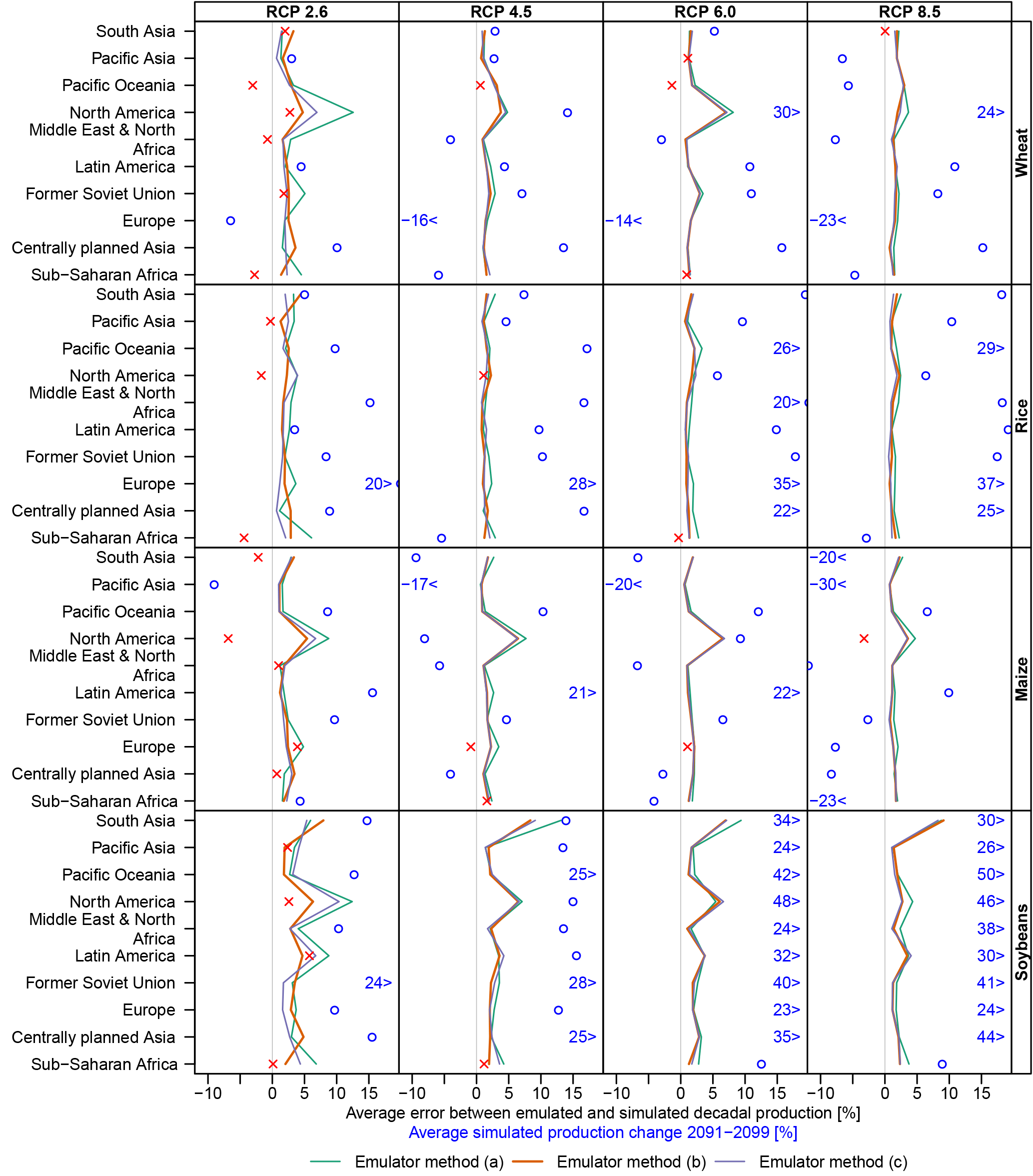
Figure 9Root-mean-square difference (as a percentage) between emulated and simulated regional decadal production (yields multiplied by year-2000 growing areas, combined for irrigated and rain-fed crops) for LPJmL forced by HadGEM2-ES climate projections. The emulator was built using all available data and used to reproduce yield changes in all four RCPs. For comparison, point symbols illustrate the average simulated yield change for 2091–2099 (same horizontal axis), using red crosses or blue circles depending on whether the error between emulated and simulated production is larger or smaller than the simulated change. Simulated yield changes outside the plot range are indicated by a number in the plot margin. Analogous figures for the other crop models are available in the Supplement.
To get a more comprehensive indication of the performance of the emulator for the whole 95-year time series (instead of just the 2.5 ∘C bin) we use all three approaches to reproduce simulated changes in crop production under RCP2.6, RCP4.5, RCP6.0, and RCP8.5, as derived for 10 large-scale world regions. Grid point yields are aggregated to the regions assuming fixed year-2000 land use and irrigation patterns. Compared to gridded yields, using production gives less weight to areas where a crop is not currently grown. Since none of the emulators are expected to capture the relatively large inter-annual variability in simulated yields, we compare simulated and emulated decadal production and calculate the RMSE over all decades of the relative difference between emulated and simulated decadal production (as a percentage) as a measure of the performance of the emulator.
Of the two approaches that estimate warming and CO2-induced effects separately, approach (b) generally provides a better performance than approach (a) (see Fig. 9 for LPJmL, Table 3 and the Supplement for all crop models, Fig. 10 for a map of the regions). Performance of all emulator approaches varies substantially among regions. There are also considerable differences among crop models. For LPJmL, emulator approach (b) provides marginally better performance for many regions than approach (c). However, this is not consistent across the emulators for the other crop models. Taking into account that approach (b) requires additional crop model simulations with fixed CO2 and that performance is mostly very similar for approaches (b) and (c), the very basic interpolation approach (c) appears to provide the best compromise between emulator performance and complexity. Note though that the average difference between emulated and simulated production over the full 95-year time series is sometimes larger than the simulated production change in 2091–2099, especially in the low warming scenarios (marked by red crosses in Fig. 9). Table 3 compares the RMSE between emulated and simulated crop production in the largest producing region of each crop for all five crop models.
Figure 10 illustrates the performance of emulator approach (c) in reproducing decadal maize production as simulated by LPJmL forced by HadGEM2-ES. Emulated yields generally follow the simulated trends, although large errors exist, e.g. in North America, which also stands out in Figs. 9 and 8. Analogous figures for all crops, emulator approaches, and crop models are available in the Supplement.
Similar to the grid point results, using only RCP8.5 to train the emulators leads to a performance loss for all emulator methods and all RCPs except RCP8.5. This performance loss is larger for approach (a) than approaches (b) and (c), and is generally highest for RCP4.5 (figures available in the Supplement).
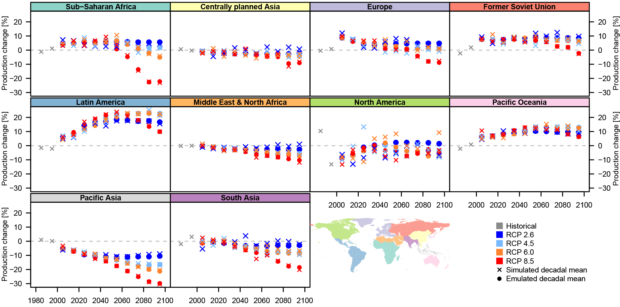
Figure 10Comparison of simulated and emulated time series of regionally aggregated crop production changes for LPJmL forced by HadGEM2-ES climate projections. Results are shown for maize and emulator approach (c). Analogous figures for the other crops, emulator approaches, and GGCMs are available in the Supplement.
In addition to estimating the yield change associated with a rise in average temperature, it is important to consider the implications of rising variance. Climate change is expected to increase not only the average temperature but also to impact the variance of temperature and precipitation, including an increase in the frequency and duration of extreme events. For this reason, when deriving simplified relationships between yield change and global climate change, it is crucial to account not only for the mean effects of rising temperature but also their concurrent implications for crop yield variance. Inter-annual yield variance can be computed for the same warming bins as used above for the average yields, which we do here for all four crops under the “no irrigation” scenario. The variance is calculated separately for the years of each RCP–GCM–GGCM combination falling into the 2.5∘C warming bin and compared to the variance of the matching GCM–GGCM combination over the historical period (1980–2010).
The global figures show broadly similar patterns across all four crops: increases in yield variability in much of the Northern Hemisphere, particularly in North America, central Asia, and China, as well as in the southern mid-latitudes (Fig. 11). The majority of model combinations projects decreasing variability in tropical regions (except for rice) as well as parts of eastern Europe; but nowhere do more than 75 % of the model combinations agree on a decrease in variability. In several instances increased variability occurs in highly productive regions such as in China for rice and the US, Brazil, and Argentina for soy. Wheat also has an increased variability in more than 50 % of the crop model simulations over the highly productive regions in China and the US. Such an increase in variability, if realized, could manifest as impacts on the price, whose volatility is tightly linked to rapid changes in supply (Gilbert and Morgan, 2010).
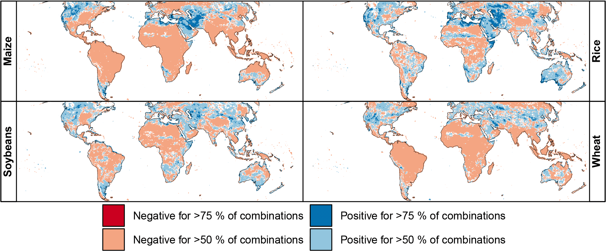
Figure 11Percentage of crop model simulations (combination of a single GCM, GGCM, and RCP scenario) in the 2.5 ∘C warming bin indicating an increase (blue) or decrease (red) in yield variance of greater than 5 % compared to the historical period (1980–2010), for maize, rice, soy, and wheat under rain-fed conditions. White indicates either a change of less than 5 % or disagreement among the models in the direction of change. Note that only four out of five GGCMs provided results for rice. An analogous figure for irrigated conditions is available in the Supplement.
Evaluating the impacts of climate change at different levels of global warming, and thus evaluating mitigation targets, requires a functional link between ΔGMT and regional impacts. Here we have shown that changes in crop yields, as simulated by gridded global crop models, can be reconstructed based on ΔGMT, with some limitations. The small spread of simulated yield change across the RCP scenarios as compared to the GCMs and impact models implies that projected impacts at different ΔGMT levels are not substantially dependent on the choice of emissions pathway. In this context, it has to be noted that the scenario setup of the ISIMIP crop model simulations was chosen specifically to minimize scenario dependency by asking modellers to keep crop management fixed at the present-day level or adjust it only in response to climate without any regard to the time horizons associated with adaptation or economic processes. Four models are calibrated to match present-day yield levels while LPJ-GUESS simulates potential yields assuming optimal management. Only two of the crop models allow for an adjustment of planting dates in response to climate change (GEPIC and PEGASUS; see Table 1). Three of the models keep the total heat unit sum to reach maturity constant, assuming no change in crop cultivar, which effectively leads to a shortening of the growing season. Representation of soil nutrient limitation varies substantially among models, with two models (LPJ-GUESS and LPJmL) considering no soil nutrient limitation at all, while the nutrients considered and the assumptions on fertilizer application differ among the other three models. The effects of these assumptions on yield changes simulated by the different crop models are not studied here since the focus of this study is on developing efficient emulators, but these assumptions inform both the simulated yield changes and the emulators which attempt to imitate the behaviour of the crop models. The results of the ISIMIP crop models have been studied in detail in Rosenzweig et al. (2014).
We have tested three different approaches for emulating crop yield change simulated by five GGCMs driven by HadGEM2-ES climate projections for four RCPs. All approaches rely on ΔGMT as the main predictor of yield change at the grid scale. Two of the approaches include pCO2 as an additional predictor. An approach (a) attributing the yield variation within an individual ΔGMT bin of a simulation with varying pCO2 solely to the change in pCO2 shows the poorest overall performance. An approach (b) based on the difference between runs with and without direct CO2 fertilization effects performs similarly well as a simple approach (c) using only ΔGMT as a single predictor. Considering the added complexity in approach (b) compared to (c), the simple approach (c) appears in general preferable even though it may not provide the best result in all regions. While our tests indicate that the emulators perform better for some crop models than for others we strongly advise against relying solely on results from any one particular model, but instead to always consider the full range of uncertainty spanned by the GGCMs. Similarly, different GCMs still account for more than 15 % of the total variance of the ISIMIP ensemble at ΔGMT = 2.5 ∘C in a number of regions (Fig. 4), which is why emulators should be constructed for all GCMs.
Given the availability of crop model simulations in the ISIMIP archive, emulators based on approaches (a) and (c) could be constructed for all five GGCMs for the remaining four GCMs (IPSL-CM5A-LR, MIROC-ESM-CHEM, GFDL-ESM2M, NorESM1-M). Emulators based on approach (b) could only be constructed for LPJmL and pDSSAT (and PEGASUS if using only RCP8.5 for training). With its five GCMs, the ISIMIP selection essentially samples as much of the CMIP5 ensemble uncertainty as is possible with such a limited subset, but still likely underestimates the total uncertainty in future climate impacts attributable to GCMs for many regions (McSweeney and Jones, 2016). The generally good performance of approach (c) suggests that simplified predictions of large-scale agricultural yields may not require additional crop model simulations with CO2 levels held at a historical level if planning to extend the GCM coverage.
While the emulators are designed to reproduce changes in average yields, the impact model ensemble assembled in this study also indicates that the variability in crop yields is projected to increase in conjunction with increasing ΔGMT in many important regions for the four major staple crops. Such an increase in yield volatility could have significant policy implications by affecting food prices and supplies, although management assumptions as well as model–structural limitations of the GGCMs to account for crop stress factors may impact the models' ability to project future changes in variability.
The scalability of mean yields is conducive to the development of predictor functions relating ΔGMT, or other aggregate climate variables readily available from simplified climate models (such as pCO2), to regional or global mean crop yield impacts. This lays the groundwork for a further exploration of the economic impacts of climate change encountered at target warming levels or over policy-relevant regions.
The coefficients estimated with Eqs. (1) to (3) are available as a Supplement, along with supplementary figures and RMSE estimates, at https://doi.org/10.5281/zenodo.1194045 (Ostberg et al., 2018). The GGCM simulations that the analysis in this paper is based on are available through https://esg.pik-potsdam.de/search/isimip-ft/ (last access: 7 May 2018), with additional documentation available on the ISIMIP website https://www.isimip.org/outputdata/caveats-fast-track/ (last access: 7 May 2018).
The supplement related to this article is available online at: https://doi.org/10.5194/esd-9-479-2018-supplement.
The authors declare that they have no conflict of interest.
This work was supported within the framework of the Leibniz Competition
(SAW-2013 PIK-5), by the EU FP7 HELIX project (grant no. 603864), and by the
German Federal Ministry for the Environment, Nature Conservation and Nuclear
Safety (16_II_148_Global_A_IMPACT). The publication of this article was
partially funded by the Open Access Fund of the Leibniz Association. For
their roles in producing, coordinating, and making the ISIMIP model output
available, we acknowledge the modelling groups (listed in
Table 1 of this paper) and the ISIMIP coordination team.
Edited by: Vivek Arora
Reviewed by: two anonymous referees
Blanc, É.: Statistical emulators of maize, rice, soybean and wheat yields from global gridded crop models, Agr. Forest Meteorol., 236, 145–161, https://doi.org/10.1016/j.agrformet.2016.12.022, 2017. a
Bondeau, A., Smith, P. C., Zaehle, S., Schaphoff, S., Lucht, W., Cramer, W., Gerten, D., Lotze-Campen, H., Müller, C., Reichstein, M., and Smith, B.: Modelling the role of agriculture for the 20th century global terrestrial carbon balance, Global Change Biol., 13, 679–706, https://doi.org/10.1111/j.1365-2486.2006.01305.x, 2007. a
Brown, M. E. and Kshirsagar, V.: Weather and international price shocks on food prices in the developing world, Global Environ. Change, 35, 31–40, https://doi.org/10.1016/j.gloenvcha.2015.08.003, 2015. a
Challinor, A. J. and Wheeler, T. R.: Crop yield reduction in the tropics under climate change: Processes and uncertainties, Agr. Forest Meteorol., 148, 343–356, https://doi.org/10.1016/j.agrformet.2007.09.015, 2008. a
Darwin, R. and Kennedy, D.: Economic effects of CO2 fertilization of crops: transforming changes in yield into changes in supply, Environ. Model. Assess., 5, 157–168, https://doi.org/10.1023/A:1019013712133, 2000. a
Deryng, D., Sacks, W. J., Barford, C. C., and Ramankutty, N.: Simulating the effects of climate and agricultural management practices on global crop yield, Global Biogeochem. Cy., 25, GB2006, https://doi.org/10.1029/2009GB003765, 2011. a
Elliott, J., Kelly, D., Chryssanthacopoulos, J., Glotter, M., Jhunjhnuwala, K., Best, N., Wilde, M., and Foster, I.: The parallel system for integrating impact models and sectors (pSIMS), Environ. Model. Softw., 62, 509–516, https://doi.org/10.1016/j.envsoft.2014.04.008, 2014. a
Eyshi Rezaei, E., Gaiser, T., Siebert, S., Sultan, B., and Ewert, F.: Combined impacts of climate and nutrient fertilization on yields of pearl millet in Niger, Eur. J. Agron., 55, 77–88, https://doi.org/10.1016/j.eja.2014.02.001, 2014. a
FAO: FertiSTAT – Fertilizer Use Statistics, Food and Agriculture Organization of the United Nations, Rome, 2007. a
Frieler, K., Meinshausen, M., Mengel, M., Braun, N., and Hare, W.: A Scaling Approach to Probabilistic Assessment of Regional Climate Change, J. Climate, 25, 3117–3144, https://doi.org/10.1175/JCLI-D-11-00199.1, 2012. a, b
Frieler, K., Levermann, A., Elliott, J., Heinke, J., Arneth, A., Bierkens, M. F. P., Ciais, P., Clark, D. B., Deryng, D., Döll, P., Falloon, P., Fekete, B., Folberth, C., Friend, A. D., Gellhorn, C., Gosling, S. N., Haddeland, I., Khabarov, N., Lomas, M., Masaki, Y., Nishina, K., Neumann, K., Oki, T., Pavlick, R., Ruane, A. C., Schmid, E., Schmitz, C., Stacke, T., Stehfest, E., Tang, Q., Wisser, D., Huber, V., Piontek, F., Warszawski, L., Schewe, J., Lotze-Campen, H., and Schellnhuber, H. J.: A framework for the cross-sectoral integration of multi-model impact projections: land use decisions under climate impacts uncertainties, Earth Syst. Dynam., 6, 447–460, https://doi.org/10.5194/esd-6-447-2015, 2015. a
Gilbert, C. L. and Morgan, C. W.: Food price volatility, Philos. T. Roy. Soc. Lond. B, 365, 3023–3034, https://doi.org/10.1098/rstb.2010.0139, 2010. a
Giorgi, F.: A Simple Equation for Regional Climate Change and Associated Uncertainty, J. Climate, 21, 1589–1604, https://doi.org/10.1175/2007JCLI1763.1, 2008. a
Golyandina, N. and Korobeynikov, A.: Basic Singular Spectrum Analysis and Forecasting with R, R package version 0.14, Comput. Stat. Data Anal., 71, 934–954, https://doi.org/10.1016/j.csda.2013.04.009, 2014. a
Golyandina, N., Korobeynikov, A., Shlemov, A., and Usevich, K.: Multivariate and 2D Extensions of Singular Spectrum Analysis with the Rssa Package, J. Stat. Softw., 67, 1–78, https://doi.org/10.18637/jss.v067.i02, 2015. a
Heinke, J., Ostberg, S., Schaphoff, S., Frieler, K., Müller, C., Gerten, D., Meinshausen, M., and Lucht, W.: A new climate dataset for systematic assessments of climate change impacts as a function of global warming, Geosci. Model Dev., 6, 1689–1703, https://doi.org/10.5194/gmd-6-1689-2013, 2013. a
Hempel, S., Frieler, K., Warszawski, L., Schewe, J., and Piontek, F.: A trend-preserving bias correction – the ISI-MIP approach, Earth Syst. Dynam., 4, 219–236, https://doi.org/10.5194/esd-4-219-2013, 2013. a
IFA: Fertilizer Use by Crop, 5th edn, International Fertilizer Industry Association (IFA), International Fertilizer Development Center (IFDC), International Potash Institute (IPI), Potash and Phosphate Institute (PPI), and Food and Agriculture Organization (FAO), Rome, 2002. a
IPCC-TGICA: General Guidelines on the Use of Scenario Data for Climate Impact and Adaptation Assessment, Tech. rep., prepared by T. R. Carter on behalf of the Intergovernmental Panel on Climate Change, Task Group on Data and Scenario Support for Impact and Climate Assessment, 2007. a
Jaggard, K. W., Qi, A., and Ober, E. S.: Possible changes to arable crop yields by 2050, Philos. T. Roy. Soc. Lon. B, 365, 2835–2851, https://doi.org/10.1098/rstb.2010.0153, 2010. a
Jones, J., Hoogenboom, G., Porter, C., Boote, K., Batchelor, W., Hunt, L., Wilkens, P., Singh, U., Gijsman, A., and Ritchie, J.: The DSSAT cropping system model, Eur. J. Agron., 18, 235–265, https://doi.org/10.1016/S1161-0301(02)00107-7, 2003. a
Kimball, B. A.: Carbon Dioxide and Agricultural Yield: An Assemblage and Analysis of 430 Prior Observations, Agron. J., 75, 779–788, https://doi.org/10.2134/agronj1983.00021962007500050014x, 1983. a
Korobeynikov, A.: Computation- and space-efficient implementation of SSA, Stat. R package version 0.14, Stat. Interface, 3, 357–368, https://doi.org/10.4310/SII.2010.v3.n3.a9, 2010. a
Lindeskog, M., Arneth, A., Bondeau, A., Waha, K., Seaquist, J., Olin, S., and Smith, B.: Implications of accounting for land use in simulations of ecosystem carbon cycling in Africa, Earth Syst. Dynam., 4, 385–407, https://doi.org/10.5194/esd-4-385-2013, 2013. a
Liu, J.: A GIS-based tool for modelling large-scale crop-water relations, Environ. Model. Softw., 24, 411–422, https://doi.org/10.1016/j.envsoft.2008.08.004, 2009. a
Liu, J., Williams, J. R., Zehnder, A. J., and Yang, H.: GEPIC – modelling wheat yield and crop water productivity with high resolution on a global scale, Agricult. Syst., 94, 478–493, https://doi.org/10.1016/j.agsy.2006.11.019, 2007. a
Lobell, D. B., Sibley, A., and Ivan Ortiz-Monasterio, J.: Extreme heat effects on wheat senescence in India, Nat. Clim. Change, 2, 186–189, https://doi.org/10.1038/nclimate1356, 2012. a, b
McSweeney, C. F. and Jones, R. G.: How representative is the spread of climate projections from the 5 CMIP5 GCMs used in ISI-MIP?, Climate Services, 1, 24–29, https://doi.org/10.1016/j.cliser.2016.02.001, 2016. a
Meinshausen, M., Smith, S. J., Calvin, K., Daniel, J. S., Kainuma, M. L. T., Lamarque, J.-F., Matsumoto, K., Montzka, S. A., Raper, S. C. B., Riahi, K., Thomson, A., Velders, G. J. M., and van Vuuren, D. P.: The RCP greenhouse gas concentrations and their extensions from 1765 to 2300, Climatic Change, 109, 213–241, https://doi.org/10.1007/s10584-011-0156-z, 2011. a
Mendelsohn, R., Basist, A., Dinar, A., Kurukulasuriya, P., and Williams, C.: What explains agricultural performance: climate normals or climate variance?, Climatic Change, 81, 85–99, https://doi.org/10.1007/s10584-006-9186-3, 2007. a
Mitchell, T. D.: Pattern scaling: an examination of the accuracy of the technique for describing future climates, Climatic Change, 60, 217–242, https://doi.org/10.1023/A:1026035305597, 2003. a
Müller, C. and Robertson, R. D.: Projecting future crop productivity for global economic modeling, Agricult. Econ., 45, 37–50, https://doi.org/10.1111/agec.12088, 2014. a, b
Müller, C., Elliott, J., and Levermann, A.: Fertilizing hidden hunger, Nat. Clim. Change, 4, 540–541, https://doi.org/10.1038/nclimate2290, 2014. a
Nelson, G. C., van der Mensbrugghe, D., Ahammad, H., Blanc, E., Calvin, K., Hasegawa, T., Havlik, P., Heyhoe, E., Kyle, P., Lotze-Campen, H., von Lampe, M., Mason d'Croz, D., van Meijl, H., Müller, C., Reilly, J., Robertson, R., Sands, R. D., Schmitz, C., Tabeau, A., Takahashi, K., Valin, H., and Willenbockel, D.: Agriculture and climate change in global scenarios: why don't the models agree, Agricult. Econ., 45, 85–101, https://doi.org/10.1111/agec.12091, 2014. a, b
Ostberg, S., Lucht, W., Schaphoff, S., and Gerten, D.: Critical impacts of global warming on land ecosystems, Earth Syst. Dynam., 4, 347–357, https://doi.org/10.5194/esd-4-347-2013, 2013. a
Ostberg, S., Schewe, J., and Frieler, K.: Fast emulator of changes in crop yields at different levels of global warming, https://doi.org/10.5281/zenodo.1194045, 2018. a, b
Oyebamiji, O. K., Edwards, N. R., Holden, P. B., Garthwaite, P. H., Schaphoff, S., and Gerten, D.: Emulating global climate change impacts on crop yields, Stat. Model., 15, 499–525, https://doi.org/10.1177/1471082X14568248, 2015. a
Parry, M., Rosenzweig, C., and Livermore, M.: Climate change, global food supply and risk of hunger, Philos. T. Roy. Soc. Lond. B, 360, 2125–2138, https://doi.org/10.1098/rstb.2005.1751, 2005. a, b
Peng, S., Huang, J., Sheehy, J. E., Laza, R. C., Visperas, R. M., Zhong, X., Centeno, G. S., Khush, G. S., and Cassman, K. G.: Rice yields decline with higher night temperature from global warming, P. Natl. Acad. Sci. USA, 101, 9971–9975, https://doi.org/10.1073/pnas.0403720101, 2004. a
Portmann, F. T., Siebert, S., and Döll, P.: MIRCA2000-Global monthly irrigated and rainfed crop areas around the year 2000: A new high-resolution data set for agricultural and hydrological modeling, Global Biogeochem. Cy., 24, GB1011, https://doi.org/10.1029/2008GB003435, 2010. a, b
Ramankutty, N., Foley, J. A., Norman, J., and McSweeney, K.: The global distribution of cultivable lands: current patterns and sensitivity to possible climate change, Global Ecol. Biogeogr., 11, 377–392, https://doi.org/10.1046/j.1466-822x.2002.00294.x, 2002. a, b
Rosenzweig, C., Elliott, J., Deryng, D., Ruane, A. C., Müller, C., Arneth, A., Boote, K. J., Folberth, C., Glotter, M., Khabarov, N., Neumann, K., Piontek, F., Pugh, T. A. M., Schmid, E., Stehfest, E., Yang, H., and Jones, J. W.: Assessing agricultural risks of climate change in the 21st century in a global gridded crop model intercomparison, P. Natl. Acad. Sci. USA, 111, 3268–3273, https://doi.org/10.1073/pnas.1222463110, 2014. a, b, c, d, e, f
Santer, B. D., Wigley, T. M., Schlesinger, M. E., and Mitchell, J. F.: Developing climate scenarios from equilibrium GCM results, Report, Max-Planck-Institut für Meteorologie, Hamburg, available at: https://www.mpimet.mpg.de/fileadmin/publikationen/Reports/Report_47.pdf (last access: 8 May 2018), report no. 47, 1–14, 1990. a
Schewe, J., Heinke, J., Gerten, D., Haddeland, I., Arnell, N. W., Clark, D. B., Dankers, R., Eisner, S., Fekete, B. M., Colón-González, F. J., Gosling, S. N., Kim, H., Liu, X., Masaki, Y., Portmann, F. T., Satoh, Y., Stacke, T., Tang, Q., Wada, Y., Wisser, D., Albrecht, T., Frieler, K., Piontek, F., Warszawski, L., and Kabat, P.: Multimodel assessment of water scarcity under climate change, P. Natl. Acad. Sci., 111, 3245–3250, https://doi.org/10.1073/pnas.1222460110, 2014. a
Schlenker, W. and Roberts, M. J.: Nonlinear temperature effects indicate severe damages to U.S. crop yields under climate change, P. Natl. Acad. Sci. USA, 106, 15594–15598, https://doi.org/10.1073/pnas.0906865106, 2009. a
Smith, P., Gregory, P. J., van Vuuren, D., Obersteiner, M., Havlík, P., Rounsevell, M., Woods, J., Stehfest, E., and Bellarby, J.: Competition for land, Philos. T. Roy. Soc. Lond. B, 365, 2941–2957, https://doi.org/10.1098/rstb.2010.0127, 2010. a
Solomon, S., Plattner, G.-K., Knutti, R., and Friedlingstein, P.: Irreversible climate change due to carbon dioxide emissions, P. Natl. Acad. Sci. USA, 106, 1704–1709, https://doi.org/10.1073/pnas.0812721106, 2009. a
Stehfest, E., van Vuuren, D., Bouwman, L., and Kram, T.: Integrated assessment of global environmental change with IMAGE 3.0: Model description and policy applications, Netherlands Environmental Assessment Agency (PBL), The Hague, 2014. a
Tadesse, G., Algieri, B., Kalkuhl, M., and von Braun, J.: Drivers and triggers of international food price spikes and volatility, Food Policy, 47, 117–128, https://doi.org/10.1016/j.foodpol.2013.08.014, 2014. a
Taylor, K. E., Stouffer, R. J., and Meehl, G. A.: An overview of CMIP5 and the experiment design, B. Am. Meteorol. Soc., 93, 485–498, https://doi.org/10.1175/BAMS-D-11-00094.1, 2012. a
van der Velde, M., Tubiello, F. N., Vrieling, A., and Bouraoui, F.: Impacts of extreme weather on wheat and maize in France: evaluating regional crop simulations against observed data, Climatic Change, 113, 751–765, https://doi.org/10.1007/s10584-011-0368-2, 2012. a
van Vuuren, D. P., Edmonds, J., Kainuma, M., Riahi, K., Thomson, A., Hibbard, K., Hurtt, G. C., Kram, T., Krey, V., Lamarque, J.-F., Masui, T., Meinshausen, M., Nakicenovic, N., Smith, S. J., and Rose, S. K.: The representative concentration pathways: an overview, Climatic Change, 109, 5–31, https://doi.org/10.1007/s10584-011-0148-z, 2011. a
Waha, K., van Bussel, L. G. J., Müller, C., and Bondeau, A.: Climate-driven simulation of global crop sowing dates, Global Ecol. Biogeogr., 21, 247–259, https://doi.org/10.1111/j.1466-8238.2011.00678.x, 2012. a
Warszawski, L., Frieler, K., Huber, V., Piontek, F., Serdeczny, O., and Schewe, J.: The Inter-Sectoral Impact Model Intercomparison Project (ISI–MIP): Project framework, P. Natl. Acad. Sci. USA, 111, 3228–3232, https://doi.org/10.1073/pnas.1312330110, 2014. a, b