the Creative Commons Attribution 4.0 License.
the Creative Commons Attribution 4.0 License.
 | 06 Apr 2018
Assessing carbon dioxide removal through global and regional ocean alkalinization under high and low emission pathways
Andrew Lenton
Richard J. Matear
David P. Keller
Vivian Scott
Naomi E. Vaughan
Atmospheric carbon dioxide (CO2) levels continue to rise, increasing the risk of severe impacts on the Earth system, and on the ecosystem services that it provides. Artificial ocean alkalinization (AOA) is capable of reducing atmospheric CO2 concentrations and surface warming and addressing ocean acidification. Here, we simulate global and regional responses to alkalinity (ALK) addition (0.25 PmolALK yr−1) over the period 2020–2100 using the CSIRO-Mk3L-COAL Earth System Model, under high (Representative Concentration Pathway 8.5; RCP8.5) and low (RCP2.6) emissions. While regionally there are large changes in alkalinity associated with locations of AOA, globally we see only a very weak dependence on where and when AOA is applied. On a global scale, while we see that under RCP2.6 the carbon uptake associated with AOA is only ∼ 60 % of the total, under RCP8.5 the relative changes in temperature are larger, as are the changes in pH (140 %) and aragonite saturation state (170 %). The simulations reveal AOA is more effective under lower emissions, therefore the higher the emissions the more AOA is required to achieve the same reduction in global warming and ocean acidification. Finally, our simulated AOA for 2020–2100 in the RCP2.6 scenario is capable of offsetting warming and ameliorating ocean acidification increases at the global scale, but with highly variable regional responses.


Atmospheric carbon dioxide (CO2) levels continue to rise as a result of human activities. Recent studies have suggested that even deep cuts in emissions may not be sufficient to avoid severe impacts on the Earth system, and the ecosystem services that it provides (Gasser et al., 2015). Recent international negotiations (UNFCCC, 2015) have agreed to limit global warming to well below 2 ∘C. The application of carbon dioxide removal (CDR), sometimes referred to as “negative emissions”, appears to be required to achieve this goal, as emission reductions alone are likely to be insufficient (Rogelj et al., 2016). In this context, there is an urgent need to assess how CDR could help either mitigate climate change or even reverse it, and to understand the potential risks and benefits of different options.
While warming represents an imminent global threat which is already significantly impacting the natural environment (Hughes et al., 2017), ocean acidification poses an additional and equally significant threat to the marine environment. At present the oceans take up about 28 % of anthropogenic CO2 emitted annually (Le Quéré et al., 2015). As CO2 is taken up by the ocean it changes its chemical equilibrium, reducing the carbonate ion concentration and decreasing pH, collectively known as ocean acidification. Furthermore, as the ocean continues to take up carbon the buffering capacity or Revelle factor (Revelle and Suess, 1957) of the seawater decreases, thereby accelerating the rate of ocean acidification.
Ocean acidification is the unavoidable consequence of rising atmospheric CO2 levels and will impact the entire marine ecosystem – from plankton at the base through to higher-trophic species at the top. Potential impacts include changes in calcification, fecundity, organism growth and physiology, species composition and distributions, food web structure, and nutrient availability (Doney et al., 2012; Fabry et al., 2008; Iglesias-Rodriguez et al., 2008; Munday et al., 2009, 2010). Within this century, the impacts of ocean acidification will increase in proportion to emissions (Gattuso et al., 2015). Furthermore, these changes will be long-lasting, persisting for centuries or longer even if emissions are halted (Frolicher and Joos, 2010).
To date, many different CDR techniques have been proposed (Shepherd et al., 2009; National Research Council, 2015). Their primary purpose is to reduce atmospheric CO2 levels, and thus most CDR methods will also reduce the impacts of ocean acidification, although some proposed techniques such as ocean pipes (Lovelock and Rapley, 2007) and micro-nutrient addition (Keller et al., 2014) may actually lead to a regional acceleration of ocean acidification in surface waters.
Artificial ocean alkalinization (AOA), through altering the chemistry of seawater, both enhances ocean carbon uptake (thereby reducing atmospheric CO2), and simultaneously reverses ocean acidification and increases the ocean's buffering capacity. AOA can be thought of as a massive acceleration of the natural processes of chemical weathering of minerals that have played a role in modulating the climate on geological timescales (Zeebe, 2012; Colbourn et al., 2015; Sigman and Boyle, 2000).
Specifically, as alkalinity enters the ocean, the pH increases leading to an elevated carbonate ion concentration, a reduction in the hydrogen ion concentration, and a decrease in the concentration of aqueous CO2 (or pCO2). This in turn enhances the disequilibrium of CO2 between the ocean and atmosphere (or ΔpCO2= pCOCO leading to increased ocean carbon uptake, and a reduction in the atmospheric CO2 concentration. These increases in pH and carbonate ion concentration thus reverse the ocean acidification due to uptake of anthropogenic CO2.
Kheshgi (1995) first proposed AOA as a method of CDR. Renforth and Henderson (2017) review the early experimental, engineering, and modelling work undertaken to investigate AOA. From the observational perspective, we draw particular attention to the experimental work of Albright et al. (2016) which provided an in situ demonstration of localized AOA to offset the observed changes in ocean acidification on the Great Barrier Reef which have occurred since the pre-industrial period.
Several modelling studies have explored the impacts of AOA both on carbon sequestration and ocean acidification. Using ocean-only biogeochemical models, Kohler et al. (2013) explored AOA via olivine addition. Olivine, in addition to increasing alkalinity also adds iron and silicic acid, both of which can enhance ocean productivity (Jickells et al., 2005; Ragueneau et al., 2000). Kohler et al. (2013) estimated the response of atmospheric CO2 levels and pH to different levels of olivine addition over the period 2000–2010, and this was later extended to 2100 by Hauck et al. (2016). These studies demonstrate a global impact that appears to scale with the amount of olivine added. Importantly, Kohler et al. (2013) showed that the global effect of alkalinity added along shipping routes (as an analogue for practical implementation) was not significantly different from that of alkalinity added in a highly idealized uniform manner.
Ilyina et al. (2013) explored the potential of AOA to mitigate rising atmospheric CO2 levels and ocean acidification in ocean-only biogeochemical simulations, and they showed that AOA has the potential to ameliorate future changes due to high CO2 emissions. They did not limit the amount of AOA, as their goal was to offset the projected future changes, and showed that the amount of AOA required to do this would drive the carbonate system to levels well above pre-industrial levels. Ilyina et al. (2013) also conclude that local AOA could potentially be used to offset the impacts of ocean acidification, with enhanced CO2 uptake being only a side benefit. This regional approach was explored further by Feng et al. (2016) who suggested that local AOA in the tropical ocean, in areas of high coral calcification, has the potential to offset the impacts of future rising atmospheric CO2 levels under a high emissions scenario (RCP8.5). This study also revealed strong regional sensitivities in the response of ocean acidification related to the locations in which it was applied.
Several other studies have estimated the response of the Earth system to AOA. Gonzalez and Ilyina (2016) used an Earth system model (ESM) to estimate the AOA required to reduce atmospheric concentrations from a high emissions scenario (RCP8.5) to the medium emissions scenario (RCP4.5). They estimated that to mitigate the associated 1.5 K warming difference, via reducing atmospheric CO2 concentrations by ∼ 400 ppm, an addition of 114 Pmol of alkalinity (between 2018 and 2100) would be required, and it would come at the cost of very large (unprecedented) changes in ocean chemistry.
Keller et al. (2014) used an Earth system model of intermediate complexity (EMIC) to explore the impacts of AOA over the period 2020–2100 arising from a globally uniform addition of alkalinity (0.25 PmolALK yr−1), an amount based on the estimated carrying capacity of global shipping following Kohler et al. (2013). Keller et al. (2014) showed that AOA led to a reduction in atmospheric CO2 of 166 PgC (or ∼ 78 ppm), a net surface air temperature cooling of 0.26 K and a global increase in ocean pH of 0.06 in the period 2020–2100.
To date, not all modelling studies have been emissions driven, and this is important as potential climate and carbon cycle feedbacks may not have been accounted for. Capturing these feedbacks is critical as they have the potential to significantly increase atmospheric CO2 concentrations (Jones et al., 2016). Further, no studies have explored the impact of AOA under low emissions scenarios such as RCP2.6. This is important because scenarios that limit warming to 2 ∘C or less, currently assume considerable land-based CDR via afforestation and/or Biomass energy with carbon capture and storage (BECCS). Furthermore, the feasibility of these approaches is increasingly questioned due in part to limited land (Smith et al., 2016), whereas the potential CDR capacity of the oceans is orders of magnitude greater (Scott et al., 2015).
In this work, we use a fully coupled ESM (CSIRO-Mk3L-COAL), which includes climate and carbon feedbacks, to investigate the impact of AOA on the carbon cycle, global surface warming (2 m surface air temperature), and the ocean acidification response to the global and regional AOA experiments under the high (RCP8.5) and low (RCP2.6) emissions scenarios.
2.1 Model description
The model simulations were performed using the CSIRO-Mk3L-COAL (Carbon, Ocean, Atmosphere, Land) ESM which includes climate–carbon interactions and feedbacks (Matear and Lenton, 2014; Q. Zhang et al., 2014). The ocean component of the ESM has a resolution of 2.8∘ by 1.6∘ with 21 vertical levels. The ocean biogeochemistry is based on Lenton and Matear (2007) and Matear and Hirst (2003) simulating the distributions of phosphate, oxygen, dissolved inorganic carbon, and alkalinity in the ocean. The model simulates particulate inorganic carbon (PIC) production as a function of particulate organic carbon (POC) production via the rain ratio (9 %) following Yamanaka and Tajika (1996). This ocean biogeochemical model was shown to simulate the observed distributions of total carbon and alkalinity in the ocean (Matear and Lenton, 2014) and phosphate (Duteil et al., 2012).
The atmosphere resolution is 5.6∘ × 3.2∘ with 18 vertical layers. The land surface scheme uses CABLE (Best et al., 2015) coupled to CASA-CNP (Wang et al., 2010; Mao et al., 2011) which simulates biogeochemical cycles of carbon, nitrogen, and phosphorus in plants and soils. The response of the land carbon cycle was shown to simulate the observed biogeochemical fluxes and pools on the land surface (Wang et al., 2010).
To quantify the changes in ocean acidification, we calculate pH changes on the total scale following the recommendation of Riebesell et al. (2010). To calculate the changes of carbonate saturation state, we use the equation of Mucci (1983).
2.2 Model experimental design
Our ESM was spun up under a pre-industrial atmospheric CO2 concentration of 284.7 ppm, until the simulated climate was stable (> 2000 years) (Phipps et al., 2012). From the spun-up initial climate state, the historical simulation (1850–2005) was performed using the historical atmospheric CO2 concentrations as prescribed by the CMIP5 simulation protocol (Taylor et al., 2012).
Following the historical concentration pathway from 2006 onward, two different future projections to 2100 were made using the atmospheric CO2 emissions corresponding to the Representative Concentration Pathways of low emissions (RCP2.6) and high emissions (RCP8.5 or “business as usual”) (Taylor et al., 2012). All simulations include the forcing due to non-CO2 greenhouse gas concentrations (Taylor et al., 2012). We define RCP8.5 and RCP2.6 as our control cases for the corresponding experiments below.
In the period 2020–2100, we undertook a number of AOA experiments using a fixed quantity of 0.25 Pmol yr−1 of alkalinity, a similar amount to that used by Keller et al. (2014). Consistent with this study, we applied AOA in the surface ocean all year round in ice-free regions, set to be between 60∘ S and 70∘ N (note that this ignores the presence of seasonal sea ice in some small regions). For each of the two emissions scenarios, we considered four different regional applications of AOA, shown in Fig. 1. These are: (i) AOA globally (AOA_G) between 60∘ S and 70∘ N; (ii) the higher latitudes comprising the subpolar Northern Hemisphere oceans (40–70∘ N) and the (ice-free) Southern Ocean (40–60∘ S) (AOA_SP); (iii) the subtropical oceans (15–40∘ N and 15–40∘ S) (AOA_ST); and (iv) in the equatorial regions (15∘ N–15∘ S) (AOA_T). In this study, we only look at the response of the Earth system to alkalinity injection. We do not consider the biogeochemical response to other minerals and elements that can be associated with the sourcing of alkalinity from the application of finely ground ultra-mafic rocks such as olivine and forsterite, nor dissolution processes required to increase alkalinity (e.g. Montserrat et al., 2017).
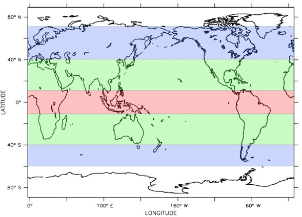
Figure 1Ocean regions used for alkalinity injection in the period 2020–2100. Blue denotes the subpolar regions (AOA_SP), green regions represent the subtropical gyres (AOA_ST), the red area represents the tropical ocean (AOA_ T), and all coloured regions combined the global alkalinity injection (AOA_ G). Note that the ocean regions not coloured represent the seasonal sea ice, where no alkalinity was added in the simulation.
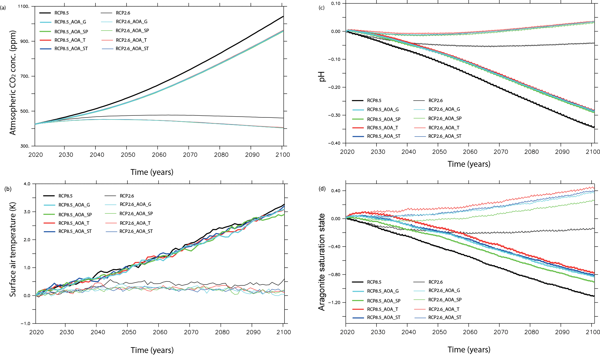
Figure 2The global mean changes in: atmospheric CO2 concentration (a), surface air temperature (SAT; b), surface ocean pH (c), and aragonite saturation state (d), for high (RCP8.5) and low emissions (RCP2.6) with global and regional AOA in the period 2020–2100.
To aid in presenting our results and to compare these with previous studies, we first discuss the carbon cycle, global surface warming (2m surface air temperature), and ocean acidification response to the four different AOA experiments under the high (RCP8.5) and low (RCP2.6) emissions scenarios. We then look at the regional behaviour of the simulations in the different AOA experiments.
3.1 Global response
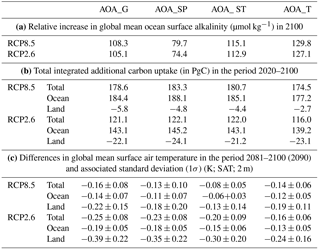
For each emissions scenario, we simulated four different AOA experiments, which all had the same 0.25 Pmol yr−1 of alkalinity added. In the case of the regional experiments the per surface values were larger than the case of global addition. As anticipated, by 2100 AOA increased the global mean surface ocean alkalinity relative to the corresponding scenario control case, with the magnitude of the increase in alkalinity being dependent on where it was added (Table 1). Subpolar addition (AOA_SP) led to the smallest net increase in surface alkalinity, while tropical addition (AOA_ T) produced the greatest increase. As expected, the global mean changes in surface alkalinity between emissions scenarios are very small (less than 3 µmol kg−1 difference). The slightly greater increase in surface values in alkalinity under RCP8.5 likely reflects enhanced ocean stratification under higher emissions (Yool et al., 2015).
Table 1For the two RCP scenarios: (a) the relative increase in global mean ocean surface alkalinity (µmol kg−1) between each AOA experiment and control experiment in 2100; (b) the total integrated additional carbon uptake (in PgC) in the period 2020–2100 in different experiment and emissions scenarios, positive denotes enhanced uptake; (c) the differences in global mean surface air temperature in the period 2081–2100 (2090) and associated standard deviation (1σ) (K; SAT; 2 m) for the four different AOA experiments for each emission scenario, relative to the same emission scenario with no AOA.
3.1.1 Carbon cycle
The large atmospheric CO2 concentration in 2100 under RCP8.5 reflects the large projected increase in emissions during this century, while under RCP2.6 a similar atmospheric concentration of CO2 is seen in 2100 as at the beginning of the simulation (2020) (Fig. 2a). We note that atmospheric CO2 levels in our CSIRO-MK3L-COAL for the control cases are greater than for their respective concentration driven RCPs due to nutrient limitation in the land, leading to reduced carbon uptake (Q. Zhang et al., 2014).
Under all emissions scenarios and experiments, AOA leads to reduced atmospheric CO2 levels (Fig. 2a). Under RCP8.5, AOA reduces atmospheric concentration by 82–86 ppm; representing a ∼ 16 % decrease in atmospheric concentration. In contrast to RCP8.5, AOA under RCP2.6 leads to a smaller reduction in atmospheric concentration (53–58 ppm). Fig. 2a shows that, by the end of the century, AOA compensates for the projected increase in atmospheric CO2 due to RCP2.6.
Over the 2020–2100 period, the reduction in atmospheric CO2 levels associated with AOA is primarily due to increased ocean carbon uptake, offset by small decreases in the land surface carbon uptake (Table 1). In the ocean, RCP8.5 leads to much greater net uptake than RCP2.6, about 50 % more, due to the larger (and growing) disequilibrium between the atmosphere and ocean.
In the ocean, the relative increase in carbon uptake in response to AOA is primarily abiotic in nature. Consistent with Keller et al. (2014) and Hauck et al. (2016) the simulated changes in ocean export production were very small (∼ 0.2 PgC) under RCP8.5, which was due to small changes in ocean state, e.g. stratification. Under RCP2.6, it was slightly larger at 1.2 PgC, but still less than 1 % percent of the total ocean uptake increase simulated under AOA, due to small changes in ocean state in a more stratified ocean. In contrast, the relative decreases in land carbon uptake were biotic in nature. The simulated cooling drove both a reduced net primary production, leading to reduced carbon uptake, and an increase in carbon retention associated with a reduction in heterotrophic respiration. However, overall, the net decrease in land carbon uptake means that in the response to AOA globally the reduced net primary production dominated. On the land, in the RCP8.5 simulation there was a smaller reduction in carbon uptake than in RCP2.6 (Table 1), due to larger decreases in surface air temperature (SAT) over land in RCP2.6 than RCP8.5 (∼ 2×; see Sect. 3.1.2). The land carbon cycle response was also smaller under high than low emissions due to nutrient limitation being reached, thereby limiting the effect of CO2 fertilization (Q. Zhang et al, 2014).
For both emissions scenarios, the four AOA experiments all produced similar reductions in atmospheric CO2 concentrations (Fig. 2) with less than a 5 % difference in the total land and ocean carbon uptake. The global changes in land and ocean carbon uptake are not very sensitive to where we add the alkalinity to the surface ocean. This is consistent with Kohler et al. (2013) who saw little difference in adding olivine along existing shipping tracks, versus uniformly adding it to the surface ocean. It is also consistent with regional addition studies of Ilyina et al. (2013), Feng et al. (2016), and Feng et al. (2017) which demonstrated a global impact.
Our simulated total increased carbon uptake under AOA_G with RCP8.5 (179 PgC) is comparable to the 166 PgC reported by Keller et al. (2014). Their cumulative increase in ocean carbon uptake by 2100 of 181 PgC is in very good agreement with our value of 184 PgC. However, they simulated a reduction in land uptake nearly twice the −5.8 PgC reduction in our AOA_G simulation. These differences reflect both the lower sensitivity of the simulated climate feedbacks in our ESM, and differences in land surface models.
3.1.2 Surface air temperature
In the control simulations, the global mean surface air temperature (SAT; 2 m) increased in the period 2020–2100 with RCP2.6 simulating a net warming of 0.4 ± 0.1 K while RCP8.5 warmed by 2.7 ± 0.1 K (2081–2100). AOA experiments simulated a reduction in global mean SAT relative to their corresponding control simulation (Fig. 2b). Within each emissions scenario the global mean SAT decline associated with AOA is always greater and more variable over the land than ocean (Table 1). In the period 2081–2100 we see larger mean changes in SAT under RCP2.6 than RCP8.5 primarily due to differences in atmospheric CO2 growth rate. Krasting et al. (2014) showed that the slower rate of emissions, the lower the radiative forcing response. This occurs in response to the timescales associated with the uptake of heat and carbon. Consequently, under RCP8.5 the atmospheric CO2 growth rate is much faster than RCP2.6, leading to a strong radiative forcing response. This explains why, despite a larger reduction in atmospheric CO2 concentration under RCP8.5, the biggest reduction in global mean SAT occur under RCP2.6. These mean changes are also associated with large inter-annual variability.
Under RCP2.6, all the AOA experiments keep global warming levels much closer to values in 2020 than RCP2.6 by the end of this century (2100; Fig. 2b). In contrast, under the RCP8.5 scenario, none of the AOA experiments have a significant impact on the projected warming by the end of this century (less than 10 %) reflecting the large warming projected under high emissions.
Within each of the scenarios, there are some differences in the magnitude of the cooling within the four different AOA experiments; however, these are smaller than the inter-annual variability over the last two decades of the simulations. Therefore, it appears that the global mean SAT decline with AOA is not very sensitive to where the alkalinity is added under either emission scenario.
The global mean cooling associated with AOA_G under RCP8.5 (−0.16 ± 0.08 K; 2081–2100) is close to the mean surface air temperature cooling of −0.26 K reported by Keller et al. (2014) for similar levels of AOA. These differences may reflect the simplified atmospheric representation of the University of Victoria (UVic) Earth system model of intermediate complexity and different climate sensitivities.
3.1.3 Ocean acidification
Here, we quantify changes in ocean acidification in terms of pH and aragonite saturation state changes. We consider these two diagnostics because they are associated with different biological impacts and are not necessarily well correlated (Lenton et al., 2016). In the future, the global mean changes in pH and aragonite saturation state will be proportional to the emissions trajectories following Gattuso et al. (2015), with the largest changes associated with the higher emissions (RCP8.5) (Fig. 2c–d). By 2100, despite the return to 2020 values of atmospheric CO2 concentration under RCP2.6 (Fig. 2), neither pH nor aragonite saturation state return to 2020 values, consistent with Mathesius et al. (2015).
In the 2020–2100 period, AOA under RCP2.6 led to much larger increases in surface pH and aragonite saturation state, more than 1.3 times, and 1.7 times that of RCP8.5, respectively (Table 2). These changes reflect the differences in the mean state associated with high and low emissions, specifically the difference between alkalinity and dissolved inorganic carbon (ALK-DIC), a proxy for ocean acidification (Lovenduski et al., 2015). As the values of DIC in the upper ocean are larger under RCP8.5 than RCP2.6, the difference between ALK and DIC (ALK-DIC) is smaller and the chemical buffering capacity of CO2 or Revelle factor (Revelle and Suess, 1957) is less. This means that, for a given addition of ALK the increase in the upper ocean DIC will always be greater under RCP8.5 due to its reduced buffering capacity. Consequently, the changes in ALK-DIC with AOA are greater under RCP2.6 than RCP8.5, which translates to greater increases in pH and aragonite saturation state.
While there was a significant difference in pH and aragonite saturation state changes with AOA between high and low emissions cases, the global mean changes for different AOA experiments within each scenario are quite similar (Table 2). The exception to this is the AOA_SP experiment, where the pH and aragonite saturation state changes are only ∼ 75 % of the change in the other AOA experiments. This reduced change in the polar region is consistent with the smaller changes in the surface ocean alkalinity values associated with AOA_SP (Table 1). These differences at higher latitudes reflect the enhanced subduction of alkalinity away from the surface ocean into the ocean interior that occurs in the high latitude oceans (Groeskamp et al., 2016).
AOA_G under RCP8.5 leads to a relative increase in pH of 0.06, which is consistent with Keller et al. (2014), while the relative increase in aragonite saturation state (0.28) is also very close to their simulated value (0.31). To put these changes into context, the estimated decrease in pH since the pre-industrial period is 0.1 units (Raven et al., 2005), and is already responsible for detectable changes in the marine environment (Albright et al., 2016).
Table 2The differences in surface value of aragonite saturation state and pH between the AOA experiments for each emission scenarios in 2100 relative to the emissions scenario with no AOA.
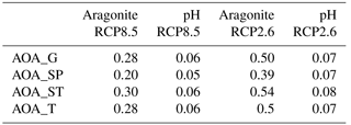
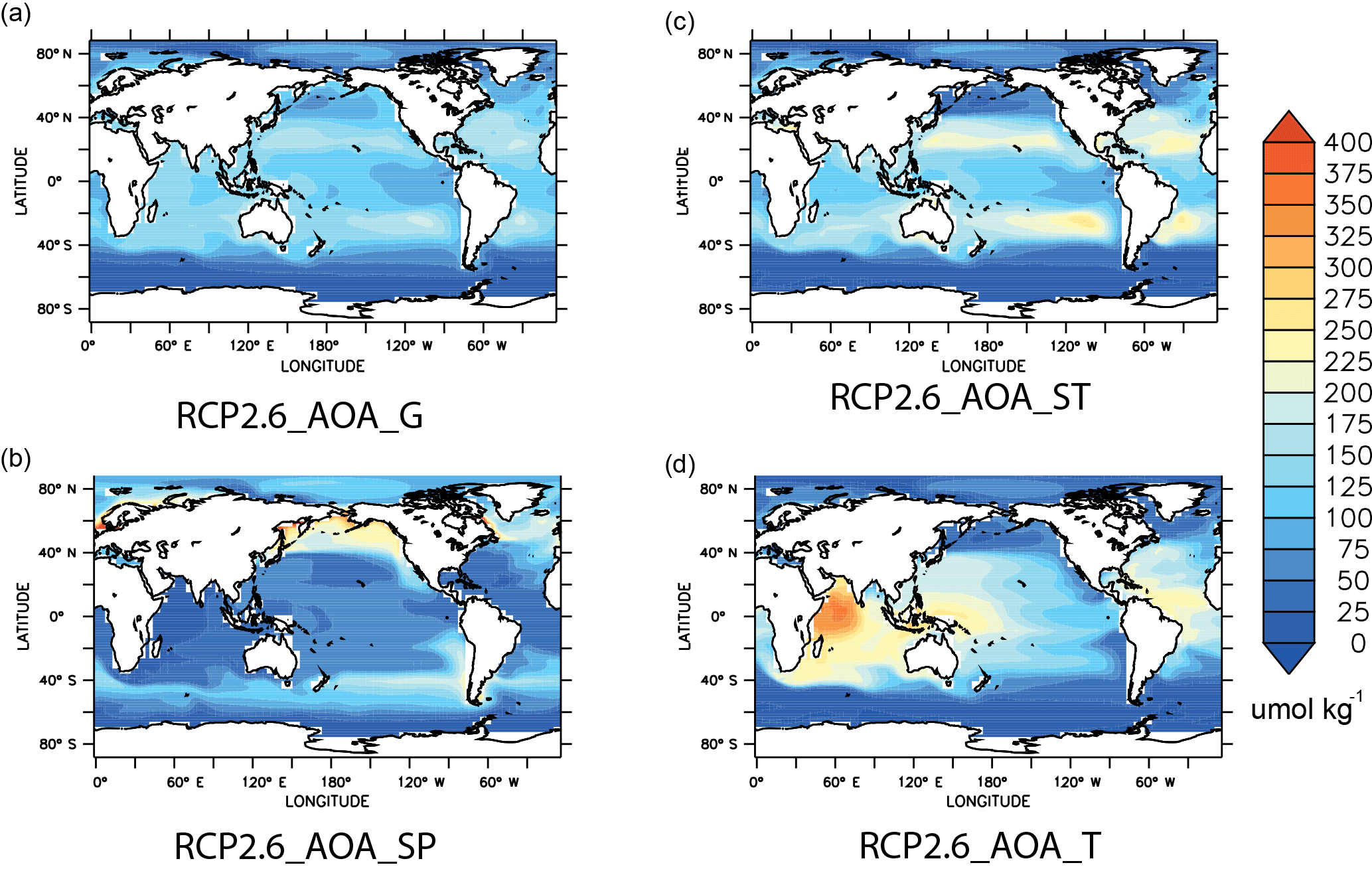
Figure 3The spatial map of the increase in surface alkalinity in 2090 (mean; 2081–2100) associated with global and regional AOA under RCP2.6 relative to RCP2.6 with no AOA. Units are µmol kg−1.
3.2 Regional responses
For both RCP scenarios, there are large regional differences in the relative surface changes in alkalinity, temperature, and ocean acidification associated with the different AOA experiments. The regional nature of these changes is closely associated with where alkalinity addition is applied, and the two different emissions scenarios considered here do not differ significantly in their behaviour. This implies that any differences in stratification and overturning circulation between the two scenarios do not significantly alter the response to AOA.
3.2.1 Surface alkalinity
For both scenarios, the greatest surface alkalinity changes occur where the alkalinity is added (Fig. 3). Spatially, under either emission scenario, the relative differences in 2090 are very similar; consequently, we only show the changes under RCP2.6 (Fig. 3). The only significant differences occur in the Arctic, reflecting larger longer-term changes in alkalinity projected under higher emissions (Yamamoto et al., 2012).
Overall, the greatest increases are seen in the tropical ocean (AOA_T) suggesting this is the most efficient region in retaining the added alkalinity in the upper ocean. This reflects the fact that subduction processes in the tropical ocean are less efficient than in other regions such as the higher latitudes. The (ice-free) subpolar oceans (AOA_ SP) produced the smallest relative increase in alkalinity, and this reflects the strong and efficient surface to interior connections through subduction occurring at higher latitudes (Groeskamp et al., 2016). The global mean relative increase associated with AOA in the subtropical gyres (AOA_ST) and globally (AOA_G) fall between the tropical (AOA_T) and higher latitude (AOA_SP) values. In the case of AOA_ST, this reflects the timescales associated with the longer residence time of upper ocean waters in the subtropical gyres.
The most modest relative increase in alkalinity occurs in the ice-covered regions where alkalinity is not explicitly added. Interestingly, even when alkalinity is added in the very high latitude Southern Ocean, it is carried northward by the Ekman current which explains the very modest increase in the region where AOA occurs between 50 and 60∘ S. In terms of the total alkalinity added to the surface ocean, about one-third remains in the upper 200 m by 2100 (Fig. 4). Specifically, for AOA_G we see that 31 % remains in the upper ocean, and for AOA_T and AOA_ST that 34 % remains in the upper ocean, while for AOA_SP the figure is 22–24 % which (as anticipated) is lower than in other regions.
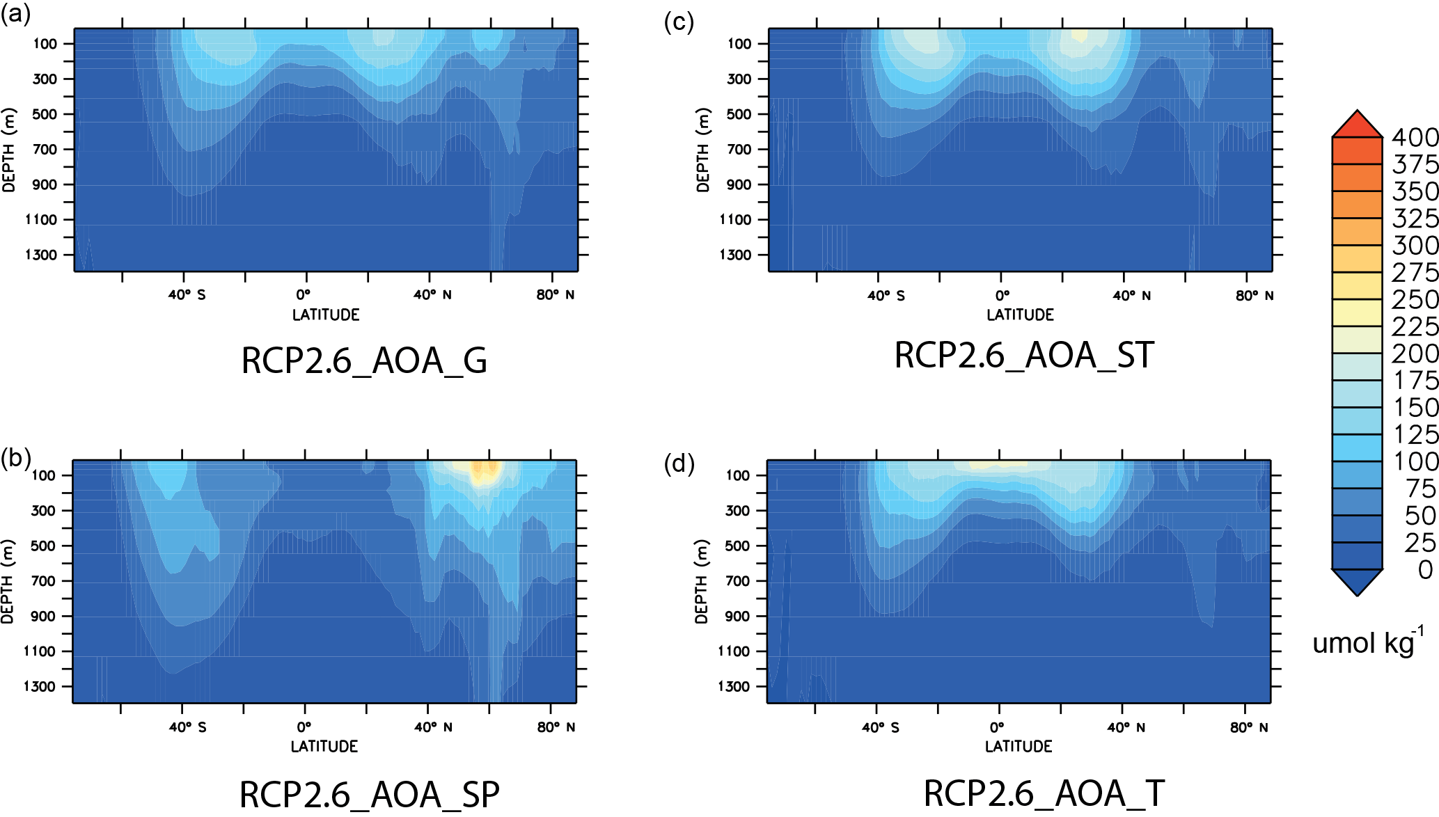
Figure 4The zonal mean changes in alkalinity in the interior ocean associated with global and regional AOA under RCP8.5 in 2090 (mean; 2081–2100) relative to RCP8.5 with no AOA. Units are µmol kg−1.
Spatially, AOA in the higher latitude regions (AOA_SP) leads to very large relative increases in alkalinity (> 1000 µmol kg−1; 2090) occurring along the northern most boundary of the northern subpolar gyres, particularly the North Pacific. Clearly, in this region the rate of AOA exceeds the rate of subduction allowing alkalinity to build up. Large relative increases in alkalinity also occur in the Southern Ocean under AOA_SP, particularly along western boundary currents. However, in contrast to northern high latitudes the values still remain low suggesting that the rate of addition does not exceed the rate of subduction even under the highest emission scenario.
AOA_ST shows a large relative increase of ∼ 300 µmol kg−1 (2081–2100) in the subtropical gyre regions. Overall, we find that these relative increases are quite homogenous across the entire subtropical gyres, with strong mixing with tropical waters leading to significant relative increases in tropical Atlantic, western Pacific and Indian Oceans. Within the tropical ocean, under AOA_T the largest relative changes are found across the entire tropical Indian Ocean (∼ 400 µmol kg−1) with large relative increases also seen in the Indonesian seas (∼ 280 µmol kg−1; 2081–2100). Away from the tropical Indian Ocean, we find that relatively homogenous increases occur in the western Pacific and the Atlantic, with much more modest relative increases in the eastern Pacific reflecting the dominant east to west upper ocean circulation. AOA_T leads to relative increases in surface alkalinity that are consistent with the response to AOA_ST – in the region of ∼ 130 µmol kg−1 (2081–2100).
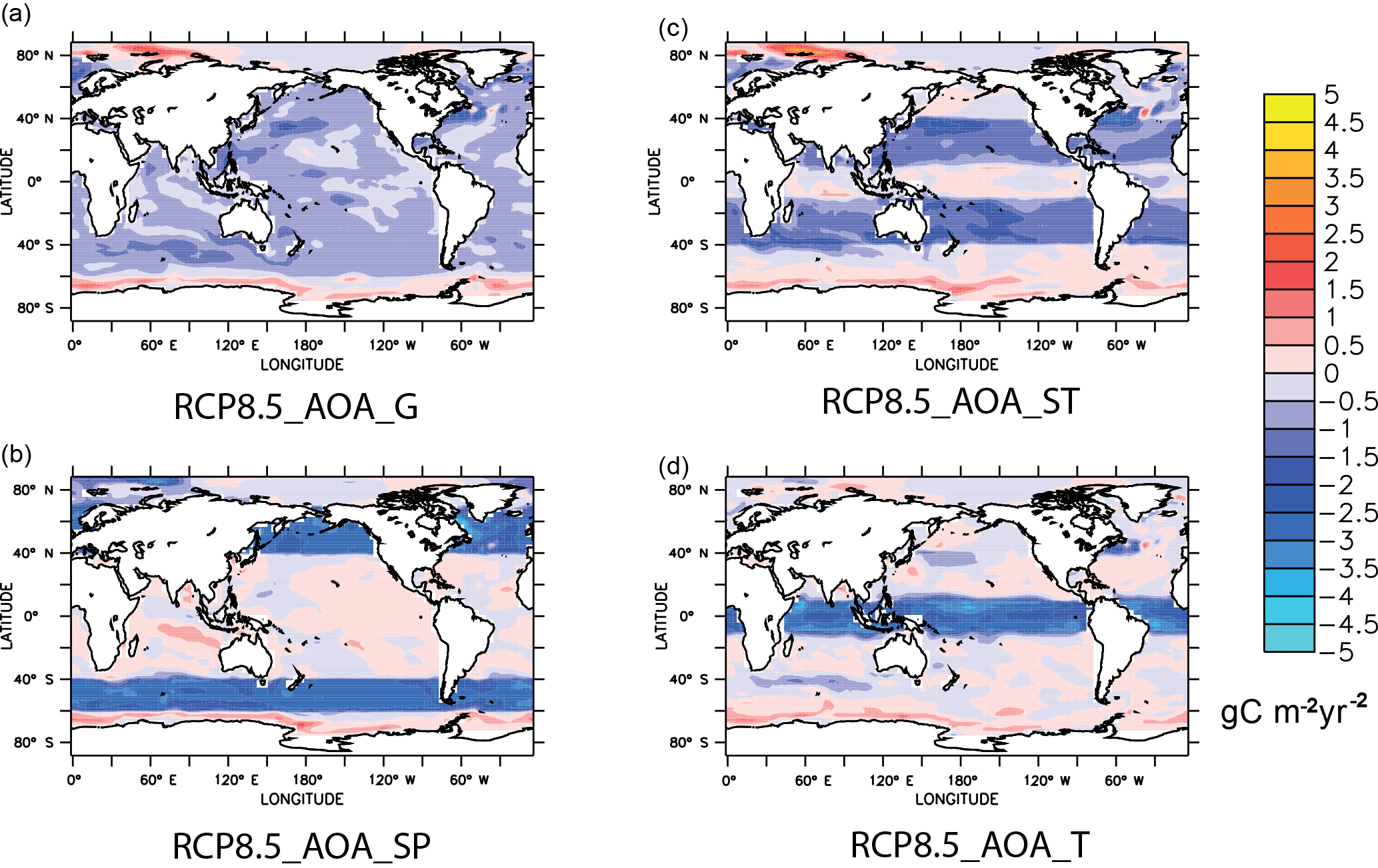
Figure 5The spatial map of the changes in ocean carbon uptake in 2090 (mean; 2081–2100) associated with global and regional AOA under RCP8.5, relative to RCP8.5 with no AOA. Units are gC m−2 yr−1.
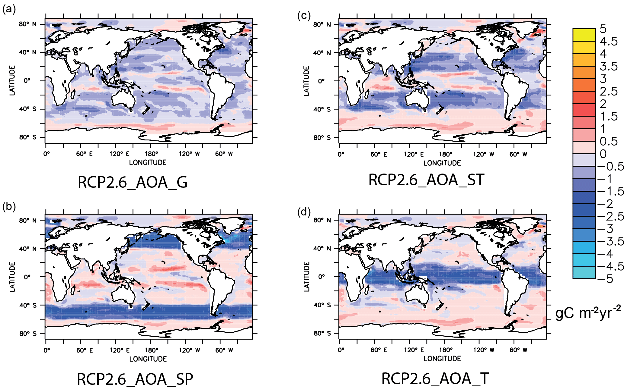
Figure 6The spatial map of the changes in ocean carbon uptake in 2090 (mean; 2081–2100) associated with global and regional AOA under RCP2.6, relative to the RCP2.6 with no AOA. Units are gC m−2 yr−1.
In the case of AOA_G, a relatively uniform net increase in alkalinity occurs in all regions with the exception of the upwelling regions such as the tropical Pacific, which showed a more modest relative increase. In AOA_G there is little evidence of any of the very large increases in alkalinity seen in the more regional AOA experiments. This spatial pattern of relative increase is broadly consistent with the pattern of global alkalinity increase simulated by Ilyina et al. (2013) and Keller et al. (2014) for AOA in the (ice-free) global ocean.
3.2.2 Changes in the interior distribution of alkalinity in the global ocean
As only about 30 % of the total AOA remains in the upper 200 m, we explore the fate of this alkalinity in the interior ocean in the zonal sections of alkalinity (Fig. 4). As the pattern is very similar between RCP2.6 and RCP8.5, we only show RCP2.6, noting that in the North Atlantic the projected ocean stratification is stronger under higher emissions (not shown) leading to slightly decreased subsurface values. This increased stratification is consistent with other studies (e.g. Yool et al., 2015).
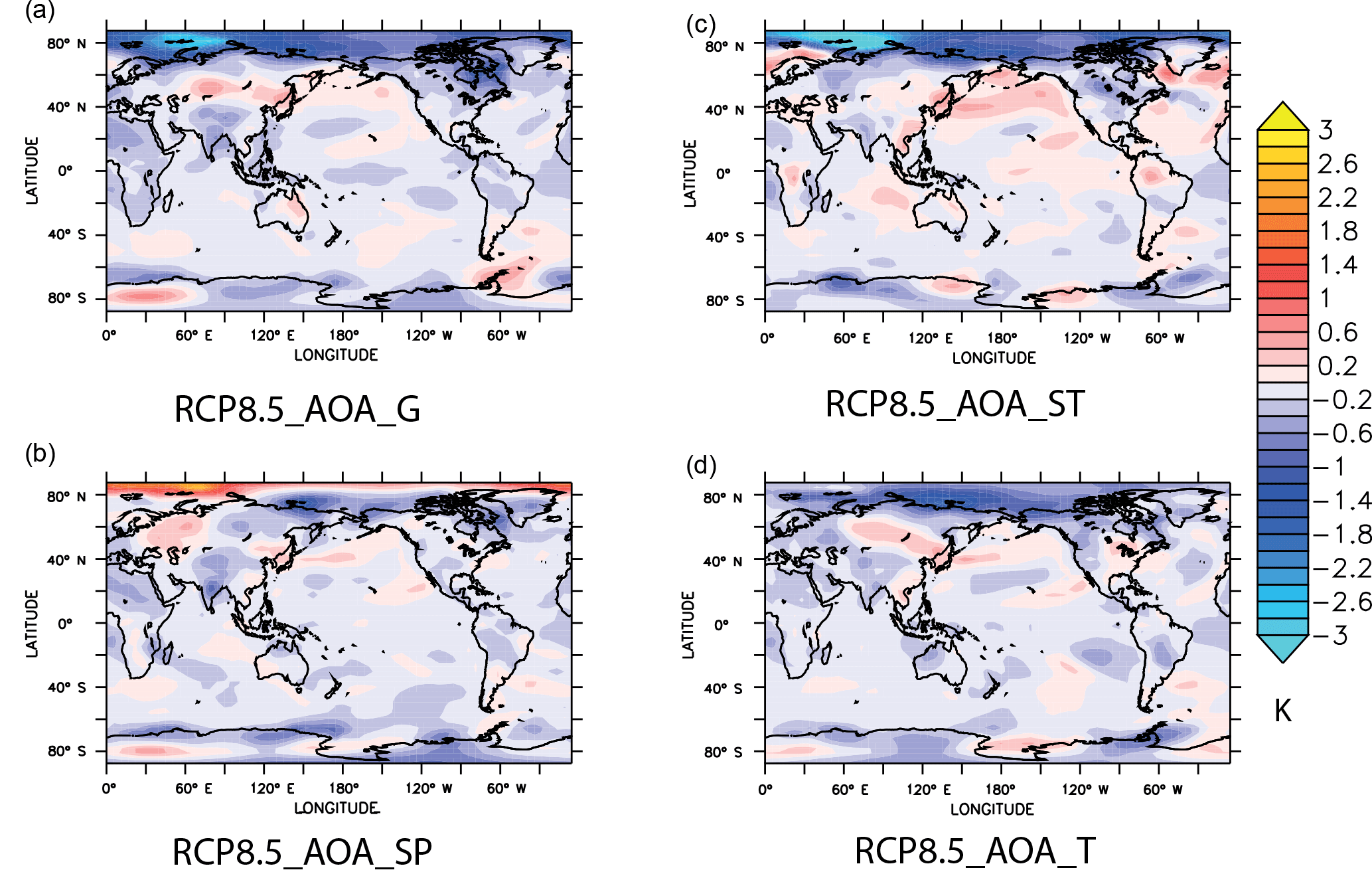
Figure 7The spatial map of the changes in surface air temperature 2090 (mean; 2081–2100) associated with global and regional AOA under RCP8.5, relative to RCP8.5 with no AOA. Units are K.
Unlike the surface plots of AOA, the relative increases in subsurface alkalinity due to AOA are very similar across all experiments. This heterogeneous spatial pattern of alkalinity increase is associated with water entering the interior ocean along specific surface to interior pathways. Alkalinity also moves into the interior ocean along the poleward boundaries of the subtropical gyres, associated with the formation and subduction of mode waters, and an increase in the subtropical gyres associated with large-scale downwelling and deep mixing in the North Atlantic. The changes in alkalinity are mainly found in the upper ocean (< 1000 m) which reflects the relatively short period of alkalinity addition. Given the short period, this is analogous to present-day observed distributions of anthropogenic carbon (Sabine et al., 2004).
As the changes in export production are very small, the large changes in the interior alkalinity concentrations primarily reflect the physical transport, rather than the sinking and remineralization of calcium carbonate. Clearly other biological processes, not represented in our model, have the potential to impact the surface and interior values of alkalinity (Matear and Lenton, 2014). One such process is the reduction in the (rain) ratio of PIC : POC under higher emissions (Riebesell et al., 2000). However, it has been shown that even a very large reduction in PIC production (50 %) would not significantly impact our results (Heinze, 2004). Unfortunately, at present the magnitude and sign of many of these other feedbacks remain poorly known (Matear and Lenton, 2014); consequently, quantifying their impact on our results is very difficult, and beyond the scope of this study.
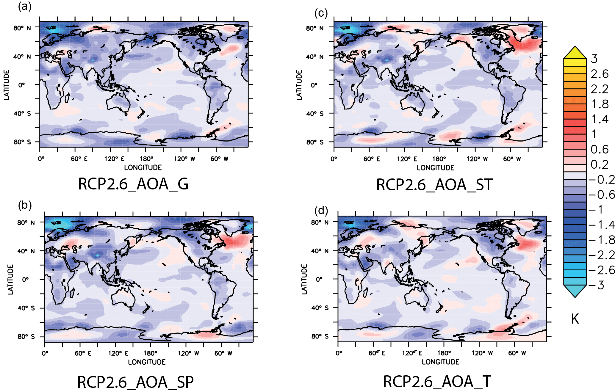
Figure 8The spatial map of the changes in surface air temperature 2090 (mean; 2081–2100) associated with global and regional AOA under RCP2.6, relative to the RCP2.6 with no AOA. Units are K.
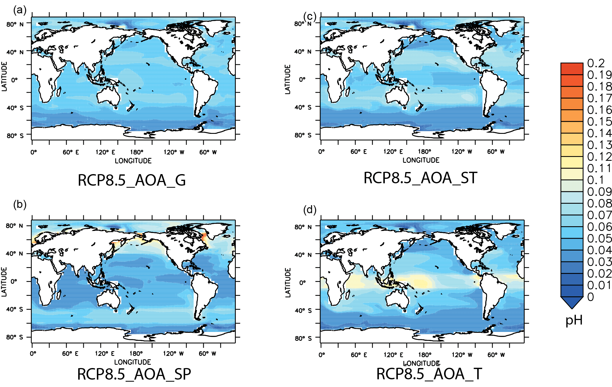
Figure 9The spatial map of the changes in pH in 2090 (mean; 2081–2100) associated with global and regional AOA under RCP8.5, relative to RCP8.5 with no AOA.
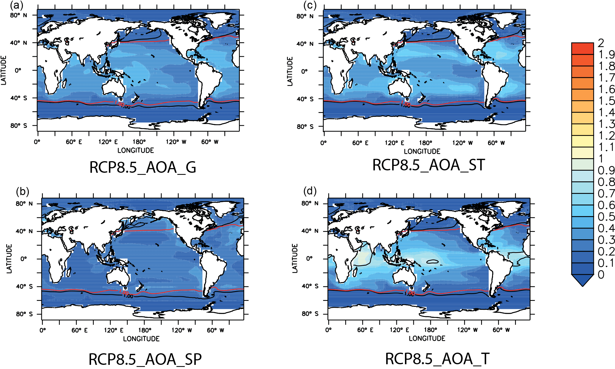
Figure 10The spatial map of the differences in surface aragonite saturation state in 2090 (mean; 2081–2100), associated with global and regional AOA under RCP8.5, relative to RCP8.5 with no AOA. Contoured on each map are the values of aragonite saturation state of 1 and 3; please see the text for more explanation. The red contours represent RCP8.5 without AOA and the black contours represent RCP8.5 with AOA for each experiment.
3.2.3 Ocean carbon cycle response
The similarity in global ocean carbon uptake associated with all AOA experiments for a given emission scenario hides the large spatial differences between simulations. Given that the largest carbon cycle response occurs in the ocean (Table 1), we focus on this response for RCP8.5 and RCP2.6 (Figs. 5 and 6). As expected, ocean carbon uptake is strongly enhanced in the regions of AOA. Away from regions of AOA, there is a reduction in carbon uptake, associated with the weakening of the gradient in CO2 between the atmosphere and ocean due to AOA. Interestingly, the largest increase spatially occurs in the Southern Ocean under AOA_SP for RCP2.6, while in contrast the largest changes under RCP8.5 occur in the tropical ocean under AOA_T. The very small changes in export production in RCP2.6 were located in the Arabian Sea (not shown), likely driven by enhanced mixing in this region. While these changes are < 1 % of the total change in carbon uptake, they may nevertheless be important regionally.
3.2.4 Temperature
The decrease in global mean SAT associated with all AOA experiments for a given emission scenario again hides the large spatial differences between the simulations. The response of surface temperature is spatially very heterogeneous (Figs. 7 and 8) and the regional surface temperature changes are very similar between the two emissions scenarios. The exception to this is the Arctic which did not show a consistent response across the different AOA experiments, reflecting the period over which the mean changes were calculated, and the simulated large variability in SAT in this region. Under both emission scenarios, the largest cooling associated with AOA occurs over northern Russia and Canada, and Antarctica (greater than a −1.5 K cooling) with a larger cooling in these regions under RCP2.6.
AOA in the RCP2.6 scenario brings about a net cooling of the surface ocean with the exception of the North Atlantic, east of New Zealand, and off the southern coast of Alaska, which show a very modest warming. A similar pattern is evident in RCP8.5; however, there is a greater cooling in the high latitudes, and less cooling in the lower latitudes than under RCP2.6.
3.2.5 Ocean acidification response
Globally, the response of pH and aragonite saturation state associated with AOA are similar; however, large spatial and regional differences are present (Figs. 9–14). To aid in the interpretation of changes in aragonite saturation state, overlain on the aragonite saturation state maps are the contours corresponding to the value of 3 – the approximate threshold for suitable coral habitat (Hoegh-Guldberg et al., 2007). On these surface maps and subsequent section plots we plot the saturation horizon, i.e. the contour corresponding to the transition from chemically stable to unstable (or corrosive), i.e. aragonite saturation state is equal to 1 (Orr et al., 2005).
The largest relative changes in pH and aragonite saturation state were associated with regions of AOA (Figs. 9–12), reflecting increases in the surface values of alkalinity (Fig. 3). All simulations increase pH and aragonite saturation state in the Arctic despite no direct addition in this region, with the largest changes here associated with AOA_G and AOA_SP. Interestingly, all simulations show little to no increase in the high latitude Southern Ocean, consistent with more efficient transport of the added alkalinity into the ocean interior.
The changes in pH associated with AOA experiments under RCP8.5, while spatially very different particularly when added in the subpolar ocean, are still much less than the decreases associated with RCP8.5 with no AOA (Fig. 9). In terms of aragonite saturation state (Fig. 10), the conditions for coral growth in the tropical ocean remain very unfavourable by the end of century (i.e. aragonite saturation state < 3) under all regional and global experiments, with the exception of AOA_T, where a very small region in the central Pacific Ocean exhibits suitable conditions.
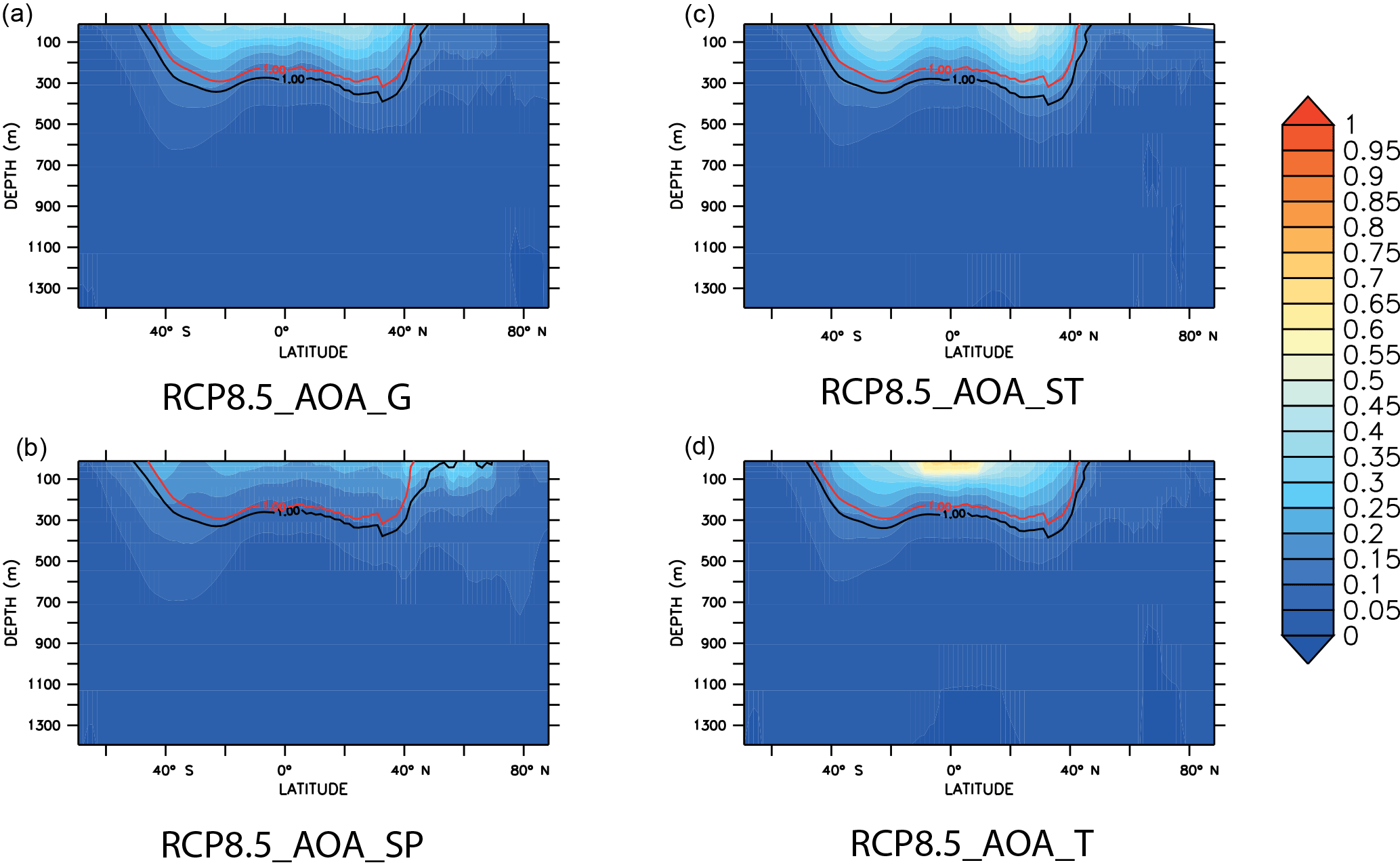
Figure 11The zonal mean differences in aragonite saturation state in 2090 (mean; 2081–2100), associated with global and regional AOA under RCP8.5, relative to RCP8.5 with no AOA. Contoured on each map are the values of aragonite saturation state of 1; please see the text for more explanation. The red contours represent RCP8.5 without AOA and the black contours represent RCP8.5 with AOA for each experiment.
Consistent with Feng et al. (2016), we find that this level of AOA under RCP8.5 is insufficient to ameliorate or significantly alter the large-scale changes in ocean acidification. More positively, at the higher latitudes the saturation horizon is moved poleward with the largest shift associated with AOA_SP, and the smallest shift at the high latitudes occurring under AOA_T. Consistent with these changes, we see a deepening of the saturation horizon everywhere, and little difference spatially between AOA experiments, consistent with zonal mean changes in alkalinity for the four AOA experiments (Fig. 11).
The spatial pattern of changes associated with AOA under RCP2.6 is broadly consistent with that seen under higher emissions; however, the magnitude of the response is much larger – again, due to the larger differences between Alkalinity and DIC with AOA under RCP2.6 (Figs. 12 and 13). In terms of aragonite saturation state, the area of tropical ocean favourable for corals is considerably expanded. As anticipated the largest changes in the area favourable for tropical corals is associated with AOA_T, closely followed by AOA_ST. As the saturation horizon does not reach the surface under RCP2.6, we can only look at the changes in the interior ocean. Here, there is a deepening in the saturation horizon of a very similar magnitude in all experiments (Fig. 14), with the exception of the Arctic. Here, the response of the saturation horizon is more sensitive to the location of the AOA, varying between ∼ 100 m under AOA_T and ∼ 280 m under AOA_SP (Fig. 14).
Spatially, the large changes in ocean acidification in response to AOA under RCP2.6 more than compensate for the changes in ocean chemistry due to low emissions in the period 2020–2100. Globally, the changes in the period 2020–2100 are sufficient to reverse or compensate for the changes since the pre-industrial period (1850). However, spatially in some regions such as equatorial upwelling, an important area of global fisheries (Chavez et al., 2003), AOA in fact leads to higher values of aragonite saturation state and pH than the ocean experienced in the pre-industrial period (Feely et al., 2009). We can only speculate on the potential impact of a reduction in aqueous CO2 and elevated pH levels on marine biota in these regions. For a recent review of the potential impact of rising pH and aragonite saturation state on marine organisms, we direct the reader to Renforth and Henderson (2017).
3.2.6 Importance of seasonality
In this paper, while we have focused on year-round AOA, as a sensitivity experiment we also explored whether AOA added in summer or winter was more efficient. To do this, we focused on the higher latitudes regions where the largest seasonal changes in mixing are found (de Boyer Montegut et al., 2004; Trull et al., 2001). Here, we tested whether AOA in either summer or winter was more effective than year-round addition. To test this for RCP8.5, we add alkalinity only during the summer at half of the annual rate (or 0.125 PmolALK yr−1) in the AOA_SP region.
Our results showed that the response to AOA in summer was very close to 50 % of the response of the year-round addition associated with AOA_SP (or 0.25 PmolALK yr−1). This suggests that the response of AOA appears invariant with regard to when the alkalinity is added. This also suggests, consistent with published studies (e.g. Keller et al., 2014; Feng et al., 2016; Kohler et al., 2013), that the response of the ocean to different quantities of AOA is scalable under the same emissions scenario. Whether this is true under very much larger additions of alkalinity, as simulated by Gonzalez and Ilyina (2016), is less clear.

Figure 12The spatial map of the changes in pH in 2090 (mean; 2081–2100) associated with global and regional AOA under RCP2.6, relative to RCP2.6 with no AOA.
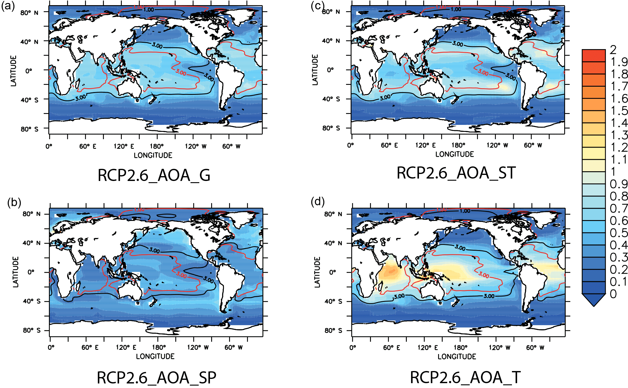
Figure 13The spatial map of the differences in surface aragonite saturation state in 2090 (mean; 2081–2100), associated with global and regional AOA under RCP2.6, relative to RCP2.6 with no AOA. Contoured on each map are the values of aragonite saturation state of 1 and 3; please see the text for more explanation. The red contours represent RCP2.6 without AOA and the black contours represent RCP2.6 with AOA for each experiment.
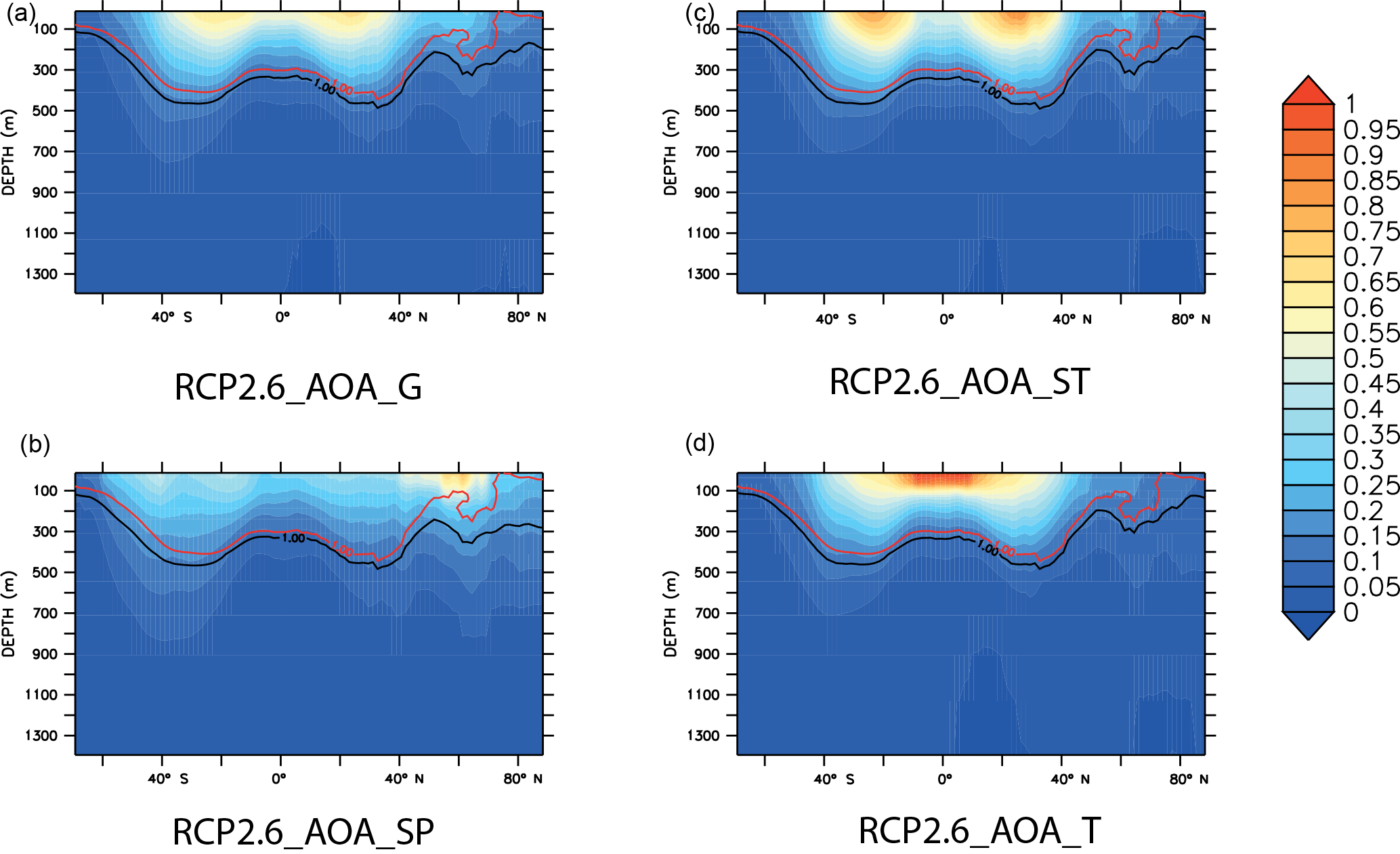
Figure 14The zonal mean differences in aragonite saturation state in 2090 (mean; 2081–2100), associated with global and regional AOA under RCP2.6, relative to RCP2.6 with no AOA. Contoured on each map are the values of aragonite saturation state of 1; please see the text for more explanation. The red contours represent RCP2.6 without AOA and the black contours represent RCP2.6 with AOA for each experiment.
Integrated Assessment modelling for the Intergovernmental Panel on Climate Change shows that CO2 removal (CDR) may be required to achieve the goal of limiting warming to well below 2 ∘C (Fuss et al., 2014). Of the many schemes that have been proposed to limit warming, only artificial ocean alkalinization (AOA) is capable of both reducing the rate and magnitude of global warming through reducing atmospheric CO2 concentrations, while simultaneously directly addressing ocean acidification. Ocean acidification, while often receiving less attention, is likely to have very long lasting and damaging impacts on the entire marine ecosystem, and the ecosystem services it provides.
Here, for the first time, we investigate the response of a fully coupled climate ESM (i.e. one that accounts for climate–carbon feedbacks) to a fixed addition of alkalinity (0.25 PmolALK yr−1) under high (RCP8.5) and low (RCP2.6) emissions scenarios. We explore the effect of global and regional application of AOA focusing on the subpolar gyres, the subtropical gyres and the tropical ocean. To assess AOA, we look at changes in surface air temperature, carbon cycling, and ocean acidification (aragonite saturation state and pH) in the period 2020–2100.
Consistent with other published studies, we see that AOA leads to reduced atmospheric CO2 concentrations, cooler global mean surface temperatures, and reduced levels of ocean acidification. Globally, for these metrics we observed that they do not vary significantly between the various AOA experiments under each emissions scenario. This implies that at the global scale there is little sensitivity of the global responses to the region where AOA is applied. We also investigate as a sensitivity experiment adding alkalinity in different seasons and see little difference in response to when AOA was undertaken.
We see under AOA that the increased carbon uptake is dominated by the ocean. Under RCP8.5, the changes due to AOA are only capable of reducing atmospheric concentrations by 16 % and, as such, the response of the climate system remains strongly dominated by warming. This is consistent with published studies of the response of the climate system under RCP8.5, and studies that have estimated the amount of AOA required to counteract a high emissions trajectory.
In contrast, AOA under RCP2.6 – while only capable of reducing atmospheric CO2 levels by 58 ppm – is sufficient to reduce atmospheric CO2 concentrations and warming to close to 2020 levels at the end of the century. This is significant as it suggests that, in combination with a rapid reduction in emissions, AOA could make an important contribution to the goal of keeping the rise in global mean temperatures below 2∘. However, AOA under the RCP2.6 emissions scenario changes the roles played by the ocean and land in carbon uptake as compared with the scenario of RCP2.6 with no AOA, resulting in a reduced uptake in the terrestrial biosphere and increased uptake in the ocean. This highlights that, while the atmospheric CO2 and warming may be reversible, the response of individual components of the Earth system to different CDR may not be (Lenton et al., 2017).
Despite the impact of AOA on the atmospheric CO2 concentration under RCP2.6 being only ∼ 60 % of the impact under RCP8.5, we see much larger changes in ocean acidification associated with RCP2.6 than RCP8.5 – more than 1.3 times in pH and more than 1.7 times in aragonite saturation state. This reflects the larger reductions in the difference between ALK and DIC that occurs under RCP2.6. We also see larger relative decreases in global temperature associated with RCP2.6. These results are very important as they demonstrate that AOA is more effective in reducing ocean acidification and global warming under lower emissions.
While there is little sensitivity in the global responses to the region in which AOA is applied, spatially the largest changes in ocean acidification (and ocean carbon uptake) were seen in the regions where AOA was applied. Despite large changes regionally, these cannot compensate for the large changes associated with RCP8.5. Even targeted AOA in the tropical ocean can preserve only a tiny area of the ocean conducive to healthy coral growth; and even then the concomitant large warming is likely to be a stronger influence on coral growth than ocean chemistry (D'Olivo and McCulloch, 2017).
In contrast, AOA under RCP2.6 is more than capable of ameliorating the projected ocean acidification changes in the period 2020–2100. We see that, in all cases, the area of the tropical ocean suitable for healthy coral growth expands, with the largest changes associated with tropical addition (AOA_T). In some areas, such as the equatorial Pacific, the changes that have occurred since the pre-industrial period are also completely reversed, and in some cases, lead to higher values of aragonite saturation state and pH than were experienced in the pre-industrial period.
While the amount of alkalinity added in this study is small in comparison to other published studies, the challenge of achieving even this level of AOA should not be underestimated. Indeed, it is not clear whether such an effort is even feasible given the cost and the logistical, political, and engineering challenges of producing and distributing such large quantities of alkaline material (Renforth and Henderson, 2017). In the case of RCP8.5, it is unlikely that this level of AOA could be justified given our results. If emissions can be reduced along an RCP2.6 type trajectory, this study suggests that AOA is much more effective and may provide a method to remove atmospheric CO2 to complement mitigation, albeit with some side-effects, and may be an alternative to reliance on land-based CDR.
In this work, and other published studies to date, we have not accounted for the role of the mesoscale in AOA. In the real ocean (mesoscale), eddies are ubiquitous and associated with strong convergent and divergent flows, and mixing plays an important role in ocean transport (Zhang et al., 2014). It is plausible that the mesoscale, and indeed fine-scale circulation in the coastal environment (e.g. Mongin et al., 2016a, b), may modulate the local response to AOA and this therefore needs to be considered in future studies.
Furthermore, this is a single model study, and the results of this work need to be tested and compared in other models. The Carbon Dioxide Removal Model Intercomparison Project (CDRMIP) was created to coordinate and advance the understanding of CDR in the Earth system (Lenton et al., 2017). CDRMIP brings together Earth system models of varying complexity in a series of coordinated multi-model experiments, one of which is a global AOA experiment (CDR_4) (Keller et al., 2018). This will allow the response of the Earth system to AOA to be further explored and quantified in a robust multi-model framework, and will examine important further questions such as including cessation effects of alkalinity addition, and the long-term fate of additional alkalinity in the ocean. In parallel, more process and observational studies (e.g. mesocosm experiments) are needed to better understand the implications of AOA.
The model code, simulations and scripts used in this study are available by contacting Andrew Lenton (andrew.lenton@csiro.au) and a persistent URL on the CSIRO data portal site https://data.csiro.au/dap will be created.
The authors declare that they have no conflict of interest.
David P. Keller acknowledges funding received from the German Research
Foundation's Priority Program 1689 “Climate Engineering” (project CDR-MIA;
KE 2149/2-1). The authors also wish to thank Tom W. Trull and the three anonymous reviewers for their helpful
comments that improved this manuscript.
Edited by: Ben Kravitz
Reviewed by: three anonymous referees
Albright, R., Caldeira, L., Hosfelt, J., Kwiatkowski, L., Maclaren, J. K., Mason, B. M., Nebuchina, Y., Ninokawa, A., Pongratz, J., Ricke, K. L., Rivlin, T., Schneider, K., Sesboue, M., Shamberger, K., Silverman, J., Wolfe, K., Zhu, K., and Caldeira, K.: Reversal of ocean acidification enhances net coral reef calcification, Nature, 531, 362–265, https://doi.org/10.1038/nature17155, 2016.
Best, M. J., Abramowitz, G., Johnson, H. R., Pitman, A. J., Balsamo, G., Boone, A., Cuntz, M., Decharme, B., Dirmeyer, P. A., Dong, J., Ek, M., Guo, Z., Haverd, V., Van den Hurk, B. J. J., Nearing, G. S., Pak, B., Peters-Lidard, C., Santanello, J. A., Stevens, L., and Vuichard, N.: The Plumbing of Land Surface Models: Benchmarking Model Performance, J. Hydrometeorol., 16, 1425–1442, https://doi.org/10.1175/JHM-D-14-0158.1, 2015.
Chavez, F. P., Ryan, J., Lluch-Cota, S. E., and Niquen, M.: From anchovies to sardines and back: Multidecadal change in the Pacific Ocean, Science, 299, 217–221, https://doi.org/10.1126/Science.1075880, 2003.
Colbourn, G., Ridgwell, A., and Lenton, T. M.: The time scale of the silicate weathering negative feedback on atmospheric CO2, Global Biogeochem. Cy., 29, 583–596, https://doi.org/10.1002/2014GB005054, 2015.
de Boyer Montegut, C., Madec, G., Fischer, A. S., Lazar, A., and Iudicone, D.: Mixed layer depth over the global ocean: An examination of profile data and a profile-based climatology, J. Geophys. Res.-Oceans, 109, C12003, https://doi.org/10.1029/2004jc002378, 2004.
D'Olivo, J. P. and McCulloch, M. T.: Response of coral calcification and calcifying fluid composition to thermally induced bleaching stress, Scientific Reports, 7, 2207, https://doi.org/10.1038/S41598-017-02306-X, 2017.
Doney, S. C., Ruckelshaus, M., Duffy, J. E., Barry, J. P., Chan, F., English, C. A., Galindo, H. M., Grebmeier, J. M., Hollowed, A. B., Knowlton, N., Polovina, J., Rabalais, N. N., Sydeman, W. J., and Talley, L. D.: Climate Change Impacts on Marine Ecosystems, Annu. Rev. Mar. Sci., 4, 11–37, https://doi.org/10.1146/Annurev-Marine-041911-111611, 2012.
Duteil, O., Koeve, W., Oschlies, A., Aumont, O., Bianchi, D., Bopp, L., Galbraith, E., Matear, R., Moore, J. K., Sarmiento, J. L., and Segschneider, J.: Preformed and regenerated phosphate in ocean general circulation models: can right total concentrations be wrong?, Biogeosciences, 9, 1797–1807, https://doi.org/10.5194/bg-9-1797-2012, 2012.
Fabry, V. J., Seibel, B. A., Feely, R. A., and Orr, J. C.: Impacts of ocean acidification on marine fauna and ecosystem processes, ICES J. Mar. Sci., 65, 414–432, https://doi.org/10.1093/Icesjms/Fsn048, 2008.
Feely, R. A., Doney, S. C., and Cooley, S. R.: Ocean Acidification: Present Conditions and Future Changes in a High-CO2 World, Oceanography, 22, 36–47, https://doi.org/10.5670/Oceanog.2009.95, 2009.
Feng, E. Y., Keller, D. P., Koeve, W., and Oschlies, A.: Could artificial ocean alkalinization protect tropical coral ecosystems from ocean acidification?, Environ. Res. Lett., 11, 074008, https://doi.org/10.1088/1748-9326/11/7/074008, 2016.
Feng, E. Y., Koeve, W., Keller, D. P., and Oschlies, A, Model-Based Assessment of the CO2 Sequestration Potential of Coastal Ocean Alkalinization, Earth's Future, 5, 1252–1266, https://doi.org/10.1002/2017EF000659, 2017.
Frolicher, T. L. and Joos, F.: Reversible and irreversible impacts of greenhouse gas emissions in multi-century projections with the NCAR global coupled carbon cycle-climate model, Clim. Dynam., 35, 1439–1459, https://doi.org/10.1007/S00382-009-0727-0, 2010.
Fuss, S., Canadell, J. G., Peters, G. P., Tavoni, M., Andrew, R. M., Ciais, P., Jackson, R. B., Jones, C. D., Kraxner, F., Nakicenovic, N., Le Quere, C., Raupach, M. R., Sharifi, A., Smith, P., and Yamagata, Y.: Commentary: Betting on Negative Emissions, Nature Climate Change, 4, 850–853, 2014.
Gasser, T., Guivarch, C., Tachiiri, K., Jones, C. D., and Ciais, P.: Negative emissions physically needed to keep global warming below 2 ∘C, Nat. Commun., 6, 7958, https://doi.org/10.1038/Ncomms8958, 2015.
Gattuso, J.-P., Magnan, A., Billé, R., Cheung, W. W. L., Howes, E. L., Joos, F., Allemand, D., Bopp, L., Cooley, S. R., Eakin, C. M., Hoegh-Guldberg, O., Kelly, R. P., Pörtner, H.-O., Rogers, A. D., Baxter, J. M., Laffoley, D., Osborn, D., Rankovic, A., Rochette, J., Sumaila, U. R., Treyer, S., and Turley, C.: Contrasting futures for ocean and society from different anthropogenic CO2 emissions scenarios, Science, 349, aac4722, https://doi.org/10.1126/science.aac4722, 2015.
Gonzalez, M. F. and Ilyina, T.: Impacts of artificial ocean alkalinization on the carbon cycle and climate in Earth system simulations, Geophys. Res. Lett., 43, 6493–6502, https://doi.org/10.1002/2016GL068576, 2016.
Groeskamp, S., Lenton, A., Matear, R., Sloyan, B. M., and Langlais, C.: Anthropogenic carbon in the oceanSurface to interior connections, Global Biogeochem. Cy., 30, 1682–1698, https://doi.org/10.1002/2016GB005476, 2016.
Hauck, J., Kohler, P., Wolf-Gladrow, D., and Volker, C.: Iron fertilisation and century-scale effects of open ocean dissolution of olivine in a simulated CO2 removal experiment, Environ. Res. Lett., 11, 024007, https://doi.org/10.1088/1748-9326/11/2/024007, 2016.
Heinze, C.: Simulating oceanic CaCO3 export production in the greenhouse, Geophys. Res. Lett., 31, L16308, https://doi.org/10.1029/2004GL020613, 2004.
Hoegh-Guldberg, O., Mumby, P. J., Hooten, A. J., Steneck, R. S., Greenfield, P., Gomez, E., Harvell, C. D., Sale, P. F., Edwards, A. J., Caldeira, K., Knowlton, N., Eakin, C. M., Iglesias-Prieto, R., Muthiga, N., Bradbury, R. H., Dubi, A., and Hatziolos, M. E.: Coral reefs under rapid climate change and ocean acidification, Science, 318, 1737–1742, https://doi.org/10.1126/science.1152509, 2007.
Hughes, T. P., Kerry, J. T., Alvarez-Noriega, M., Alvarez-Romero, J. G., Anderson, K. D., Baird, A. H., Babcock, R. C., Beger, M., Bellwood, D. R., Berkelmans, R., Bridge, T. C., Butler, I. R., Byrne, M., Cantin, N. E., Comeau, S., Connolly, S. R., Cumming, G. S., Dalton, S. J., Diaz-Pulido, G., Eakin, C. M., Figueira, W. F., Gilmour, J. P., Harrison, H. B., Heron, S. F., Hoey, A. S., Hobbs, J. P. A., Hoogenboom, M. O., Kennedy, E. V., Kuo, C. Y., Lough, J. M., Lowe, R. J., Liu, G., Cculloch, M. T. M., Malcolm, H. A., Mcwilliam, M. J., Pandolfi, J. M., Pears, R. J., Pratchett, M. S., Schoepf, V., Simpson, T., Skirving, W. J., Sommer, B., Torda, G., Wachenfeld, D. R., Willis, B. L., and Wilson, S. K.: Global warming and recurrent mass bleaching of corals, Nature, 543, 373–377, https://doi.org/10.1038/nature21707, 2017.
Iglesias-Rodriguez, M. D., Halloran, P. R., Rickaby, R. E. M., Hall, I. R., Colmenero-Hidalgo, E., Gittins, J. R., Green, D. R. H., Tyrrell, T., Gibbs, S. J., von Dassow, P., Rehm, E., Armbrust, E. V., and Boessenkool, K. P.: Phytoplankton calcification in a high-CO2 world, Science, 320, 336–340, https://doi.org/10.1126/Science.1154122, 2008.
Ilyina, T., Wolf-Gladrow, D., Munhoven, G., and Heinze, C.: Assessing the potential of calcium-based artificial ocean alkalinization to mitigate rising atmospheric CO2 and ocean acidification, Geophys. Res. Lett., 40, 5909–5914, https://doi.org/10.1002/2013GL057981, 2013.
Jickells, T. D., An, Z. S., Andersen, K. K., Baker, A. R., Bergametti, G., Brooks, N., Cao, J. J., Boyd, P. W., Duce, R. A., Hunter, K. A., Kawahata, H., Kubilay, N., laRoche, J., Liss, P. S., Mahowald, N., Prospero, J. M., Ridgwell, A. J., Tegen, I., and Torres, R.: Global iron connections between desert dust, ocean biogeochemistry, and climate, Science, 308, 67–71, https://doi.org/10.1126/Science.1105959, 2005.
Jones, C. D., Arora, V., Friedlingstein, P., Bopp, L., Brovkin, V., Dunne, J., Graven, H., Hoffman, F., Ilyina, T., John, J. G., Jung, M., Kawamiya, M., Koven, C., Pongratz, J., Raddatz, T., Randerson, J. T., and Zaehle, S.: C4MIP – The Coupled Climate–Carbon Cycle Model Intercomparison Project: experimental protocol for CMIP6, Geosci. Model Dev., 9, 2853–2880, https://doi.org/10.5194/gmd-9-2853-2016, 2016.
Keller, D. P., Feng, E. Y., and Oschlies, A.: Potential climate engineering effectiveness and side effects during a high carbon dioxide-emission scenario, Nat. Commun., 5, 3304, https://doi.org/10.1038/Ncomms4304, 2014.
Keller, D. P., Lenton, A., Scott, V., Vaughan, N. E., Bauer, N., Ji, D., Jones, C. D., Kravitz, B., Muri, H., and Zickfeld, K.: The Carbon Dioxide Removal Model Intercomparison Project (CDRMIP): rationale and experimental protocol for CMIP6, Geosci. Model Dev., 11, 1133–1160, https://doi.org/10.5194/gmd-11-1133-2018, 2018.
Kheshgi, H. S.: Sequestering Atmospheric Carbon-Dioxide by Increasing Ocean Alkalinity, Energy, 20, 915–922, https://doi.org/10.1016/0360-5442(95)00035-F, 1995.
Kohler, P., Abrams, J. F., Volker, C., Hauck, J., and Wolf-Gladrow, D. A.: Geoengineering impact of open ocean dissolution of olivine on atmospheric CO2, surface ocean pH and marine biology, Environ. Res. Lett., 8, https://doi.org/10.1088/1748-9326/8/1/014009, 2013.
Krasting, J. P., Dunne, J. P., Shevliakova, E., and Stouffer, R. J.: Trajectory sensitivity of the transient climate response to cumulative carbon emissions, Geophys. Res. Lett., 41, 2520–2527, https://doi.org/10.1002/2013gl059141, 2014.
Lenton, A. and Matear, R. J.: Role of the Southern Annular Mode (SAM) in Southern Ocean CO2 uptake, Global Biogeochem. Cy., 21, https://doi.org/10.1029/2006GB002714, 2007.
Lenton, A., Tilbrook, B., Matear, R. J., Sasse, T. P., and Nojiri, Y.: Historical reconstruction of ocean acidification in the Australian region, Biogeosciences, 13, 1753–1765, https://doi.org/10.5194/bg-13-1753-2016, 2016.
Lenton, A., Keller, D. P., and Pfister, P.: How Will Earth Respond to Plans for Carbon Dioxide Removal?, EOS, 98, https://doi.org/10.1029/2017EO068385, 2017.
Le Quéré, C., Moriarty, R., Andrew, R. M., Peters, G. P., Ciais, P., Friedlingstein, P., Jones, S. D., Sitch, S., Tans, P., Arneth, A., Boden, T. A., Bopp, L., Bozec, Y., Canadell, J. G., Chini, L. P., Chevallier, F., Cosca, C. E., Harris, I., Hoppema, M., Houghton, R. A., House, J. I., Jain, A. K., Johannessen, T., Kato, E., Keeling, R. F., Kitidis, V., Klein Goldewijk, K., Koven, C., Landa, C. S., Landschützer, P., Lenton, A., Lima, I. D., Marland, G., Mathis, J. T., Metzl, N., Nojiri, Y., Olsen, A., Ono, T., Peng, S., Peters, W., Pfeil, B., Poulter, B., Raupach, M. R., Regnier, P., Rödenbeck, C., Saito, S., Salisbury, J. E., Schuster, U., Schwinger, J., Séférian, R., Segschneider, J., Steinhoff, T., Stocker, B. D., Sutton, A. J., Takahashi, T., Tilbrook, B., van der Werf, G. R., Viovy, N., Wang, Y.-P., Wanninkhof, R., Wiltshire, A., and Zeng, N.: Global carbon budget 2014, Earth Syst. Sci. Data, 7, 47–85, https://doi.org/10.5194/essd-7-47-2015, 2015.
Lovelock, J. E. and Rapley, C. G.: Ocean pipes could help the Earth to cure itself, Nature, 449, 403–403, https://doi.org/10.1038/449403a, 2007.
Lovenduski, N. S., Long, M. C., and Lindsay, K.: Natural variability in the surface ocean carbonate ion concentration, Biogeosciences, 12, 6321–6335, https://doi.org/10.5194/bg-12-6321-2015, 2015.
Mao, J., Phipps, S. J., Pitman, A. J., Wang, Y. P., Abramowitz, G., and Pak, B.: The CSIRO Mk3L climate system model v1.0 coupled to the CABLE land surface scheme v1.4b: evaluation of the control climatology, Geosci. Model Dev., 4, 1115–1131, https://doi.org/10.5194/gmd-4-1115-2011, 2011.
Matear, R. J. and Hirst, A. C.: Long term changes in dissolved oxygen concentrations in the ocean caused by protracted global warming, Global Biogeochem. Cy., 17, 1125, https://doi.org/10.1029/2002GB001997, 2003.
Matear, R. J. and Lenton, A.: Quantifying the impact of ocean acidification on our future climate, Biogeosciences, 11, 3965–3983, https://doi.org/10.5194/bg-11-3965-2014, 2014.
Mathesius, S., Hofmann, M., Caldeira, K., and Schellnhuber, H. J.: Long-term response of oceans to CO2 removal from the atmosphere, Nature Climate Change, 5, 1107–1113, https://doi.org/10.1038/NCLIMATE2729, 2015.
Mongin, M., Baird, M. E., Hadley, S., and Lenton, A.: Optimising reef-scale CO2 removal by seaweed to buffer ocean acidification, Environ. Res. Lett., 11, 034023, https://doi.org/10.1088/1748-9326/11/3/034023, 2016a.
Mongin, M., Baird, M. E., Tilbrook, B., Matear, R. J., Lenton, A., Herzfeld, M., Wild-Allen, K., Skerratt, J., Margvelashvili, N., Robson, B. J., Duarte, C. M., Gustafsson, M. S. M., Ralph, P. J., and Steven, A. D. L.: The exposure of the Great Barrier Reef to ocean acidification, Nat. Commun., 7, 10732, https://doi.org/10.1038/Ncomms10732, 2016b.
Montserrat, F., Renforth, P., Hartmann, J., Leermakers, M., Knops, P., and Meysman, F. J. R.: Olivine Dissolution in Seawater: Implications for CO2 Sequestration through Enhanced Weathering in Coastal Environments, Environ. Sci. Technol., 51, 3960–3972, https://doi.org/10.1021/acs.est.6b05942, 2017.
Mucci, A.: The Solubility of Calcite and Aragonite in Seawater at Various Salinities, Temperatures, and One Atmosphere Total Pressure, Am. J. Sci., 283, 780–799, 1983.
Munday, P. L., Donelson, J. M., Dixson, D. L., and Endo, G. G. K.: Effects of ocean acidification on the early life history of a tropical marine fish, P. Roy. Soc. B-Biol. Sci., 276, 3275–3283, https://doi.org/10.1098/Rspb.2009.0784, 2009.
Munday, P. L., Dixson, D. L., McCormick, M. I., Meekan, M., Ferrari, M. C. O., and Chivers, D. P.: Replenishment of fish populations is threatened by ocean acidification, P. Natl. Acad. Sci. USA, 107, 12930–12934, https://doi.org/10.1073/Pnas.1004519107, 2010.
National Research Council: Climate Intervention: Carbon Dioxide Removal and Reliable Sequestration, Washington, DC, The National Academies Press, available at: https://doi.org/10.17226/18805 (last access: 3 April 2018), 2015.
Orr, J. C., Fabry, V. J., Aumont, O., Bopp, L., Doney, S. C., Feely, R. A., Gnanadesikan, A., Gruber, N., Ishida, A., Joos, F., Key, R. M., Lindsay, K., Maier-Reimer, E., Matear, R., Monfray, P., Mouchet, A., Najjar, R. G., Plattner, G. K., Rodgers, K. B., Sabine, C. L., Sarmiento, J. L., Schlitzer, R., Slater, R. D., Totterdell, I. J., Weirig, M. F., Yamanaka, Y., and Yool, A.: Anthropogenic ocean acidification over the twenty-first century and its impact on calcifying organisms, Nature, 437, 681–686, 2005.
Phipps, S. J., Rotstayn, L. D., Gordon, H. B., Roberts, J. L., Hirst, A. C., and Budd, W. F.: The CSIRO Mk3L climate system model version 1.0 – Part 2: Response to external forcings, Geosci. Model Dev., 5, 649–682, https://doi.org/10.5194/gmd-5-649-2012, 2012.
Ragueneau, O., Treguer, P., Leynaert, A., Anderson, R. F., Brzezinski, M. A., DeMaster, D. J., Dugdale, R. C., Dymond, J., Fischer, G., Francois, R., Heinze, C., Maier-Reimer, E., Martin-Jezequel, V., Nelson, D. M., and Queguiner, B.: A review of the Si cycle in the modem ocean: recent progress and missing gaps in the application of biogenic opal as a paleoproductivity proxy, Global Planet. Change, 26, 317–365, https://doi.org/10.1016/S0921-8181(00)00052-7, 2000.
Raven, J., Caldeira, K., Elderfield, H., Hoegh-Guldberg, O., Liss, P., and Riebesell, U.: Ocean acidification due to increasing atmospheric carbon dioxide, The Royal Society, Policy Document, London, UK, 2005.
Renforth, P. and Henderson, G.: Assessing ocean alkalinity for carbon sequestration, Rev. Geophys., 55, 636–674, https://doi.org/10.1002/2016RG000533, 2017.
Revelle, R. and Suess, H. E.: Carbon dioxide exchange between atmosphere and ocean and the question of an increase of atmospheric CO2 during the past decades, Tellus, 9, 18–27, 1957.
Riebesell, U., Zondervan, I., Rost, B., Tortell, P. D., Zeebe, R. E., and Morel, F. M. M.: Reduced calcification of marine plankton in response to increased atmospheric CO2, Nature, 407, 364–367, 2000.
Riebesell, U., Fabry, V. J., Hansson, L., and Gattuso, J.-P.: Guide to best practices for ocean acidification research and data reporting, Publications Office of the European Union, Luxembourg, 260, 2010.
Rogelj, J., den Elzen, M., Hohne, N., Fransen, T., Fekete, H., Winkler, H., Chaeffer, R. S., Ha, F., Riahi, K., and Meinshausen, M.: Paris Agreement climate proposals need a boost to keep warming well below 2 ∘C, Nature, 534, 631–639, https://doi.org/10.1038/nature18307, 2016.
Sabine, C. L., Feely, R. A., Gruber, N., Bullister, J. L., Wanninkhof, R., Wong, C. S., Wallace, D. W. R., Tilbrook, B., Millero, F. J., Peng, T.-H., Kozyr, A., Ono, T., and Rios, A. F.: The Oceanic Sink for Anthropogenic CO2, Science, 305, 367–371, 2004.
Scott, V., Haszeldine, R. S., Tett, S. F. B., and Oschlies, A.: Fossil fuels in a trillion tonne world, Nature Climate Change, 5, 419–423, https://doi.org/10.1038/NCLIMATE2578, 2015.
Shepherd, J. G., Caldeira, K., Cox, P., Haigh, J., Keith, D., Launder, B. E., Mace, G., MacKerron, G., Pyle, J., Raynor, S., Redgwell, C., and Watson, A.: Geoengineering the Climate: Science, governance and uncertainty, London, The Royal Society Publishing, 82 pp., 2009.
Sigman, D. M. and Boyle, E. A.: Glacial/interglacial variations in atmospheric carbon dioxide, Nature, 407, 859–869, https://doi.org/10.1038/35038000, 2000.
Smith, P., Davis, S. J., Creutzig, F., Fuss, S., Minx, J., Gabrielle, B., Kato, E., Jackson, R. B., Cowie, A., Kriegler, E., van Vuuren, D. P., Rogelj, J., Ciais, P., Milne, J., Canadell, J. G., McCollum, D., Peters, G., Andrew, R., Krey, V., Shrestha, G., Friedlingstein, P., Gasser, T., Grubler, A., Heidug, W. K., Jonas, M., Jones, C. D., Kraxner, F., Littleton, E., Lowe, J., Moreira, J. R., Nakicenovic, N., Obersteiner, M., Patwardhan, A., Rogner, M., Rubin, E., Sharifi, A., Torvanger, A., Yamagata, Y., Edmonds, J., and Cho, Y.: Biophysical and economic limits to negative CO2 emissions, Nature Climate Change, 6, 42–50, https://doi.org/10.1038/NCLIMATE2870, 2016.
Taylor, K. E., Stouffer, R. J., and Meehl, G. A.: An Overview of CMIP5 and the Experiment Design, B. Am. Meteorol. Soc., 93, 485–498, https://doi.org/10.1175/BAMS-D-11-00094.1, 2012.
Trull, T. W., Rintoul, S. R., Hadfield, M., and Abraham, E. R.: Circulation and seasonal evolution of polar waters south of Australia: Implications for iron fertilizations for the Southern Ocean, Deep-Sea Res. Pt. II, 48, 2439–2466, 2001.
United Nations Framework on Climate Change (UNFCCC): Adoption of the Paris Agreement, 21st Conference of the Parties, available at: https://unfccc.int/resource/docs/2015/cop21/eng/l09r01.pdf (last access: 3 April 2018), 2015.
Wang, Y. P., Law, R. M., and Pak, B.: A global model of carbon, nitrogen and phosphorus cycles for the terrestrial biosphere, Biogeosciences, 7, 2261–2282, https://doi.org/10.5194/bg-7-2261-2010, 2010.
Yamamoto, A., Kawamiya, M., Ishida, A., Yamanaka, Y., and Watanabe, S.: Impact of rapid sea-ice reduction in the Arctic Ocean on the rate of ocean acidification, Biogeosciences, 9, 2365–2375, https://doi.org/10.5194/bg-9-2365-2012, 2012.
Yamanaka, Y. and Tajika, E.: The role of vertical fluxes of particulate organic material and calcite in the oceanic carbon cycle: Studies using a ocean biogeochemical general; circulation model, Global Biogeochem. Cy., 10, 361–382, 1996.
Yool, A., Popova, E. E., and Coward, A. C.: Future change in ocean productivity: Is the Arctic the new Atlantic?, J. Geophys. Res.-Oceans, 120, 7771–7790, https://doi.org/10.1002/2015JC011167, 2015.
Zeebe, R. E.: History of Seawater Carbonate Chemistry, Atmospheric CO2, and Ocean Acidification, Annu. Rev. Earth Pl. Sc., 40, 141–165, https://doi.org/10.1146/annurev-earth-042711-105521, 2012.
Zhang, Q., Wang, Y. P., Matear, R. J., Pitman, A. J., and Dai, Y. J.: Nitrogen and phosphorous limitations significantly reduce future allowable CO2 emissions, Geophys. Res. Lett., 41, 632–637, https://doi.org/10.1002/2013GL058352, 2014.
Zhang, Z. G., Wang, W., and Qiu, B.: Oceanic mass transport by mesoscale eddies, Science, 345, 322–324, https://doi.org/10.1126/science.1252418, 2014.