the Creative Commons Attribution 4.0 License.
the Creative Commons Attribution 4.0 License.
 | 16 Jan 2018
Process-level improvements in CMIP5 models and their impact on tropical variability, the Southern Ocean, and monsoons
Colin Jones
Veronika Eyring
Martin Evaldsson
Stefan Hagemann
Jarmo Mäkelä
Gill Martin
Romain Roehrig
Shiyu Wang
The performance of updated versions of the four earth system models (ESMs) CNRM, EC-Earth, HadGEM, and MPI-ESM is assessed in comparison to their predecessor versions used in Phase 5 of the Coupled Model Intercomparison Project. The Earth System Model Evaluation Tool (ESMValTool) is applied to evaluate selected climate phenomena in the models against observations. This is the first systematic application of the ESMValTool to assess and document the progress made during an extensive model development and improvement project. This study focuses on the South Asian monsoon (SAM) and the West African monsoon (WAM), the coupled equatorial climate, and Southern Ocean clouds and radiation, which are known to exhibit systematic biases in present-day ESMs.
The analysis shows that the tropical precipitation in three out of four models is clearly improved. Two of three updated coupled models show an improved representation of tropical sea surface temperatures with one coupled model not exhibiting a double Intertropical Convergence Zone (ITCZ). Simulated cloud amounts and cloud–radiation interactions are improved over the Southern Ocean. Improvements are also seen in the simulation of the SAM and WAM, although systematic biases remain in regional details and the timing of monsoon rainfall. Analysis of simulations with EC-Earth at different horizontal resolutions from T159 up to T1279 shows that the synoptic-scale variability in precipitation over the SAM and WAM regions improves with higher model resolution. The results suggest that the reasonably good agreement of modeled and observed mean WAM and SAM rainfall in lower-resolution models may be a result of unrealistic intensity distributions.
- Article
(16751 KB) - Full-text XML
-
Supplement
(1137 KB) - BibTeX
- EndNote


Despite the progress made in the past, global climate models (GCMs) and earth system models (ESMs) still show significant systematic biases in a number of key features of the simulated climate system compared with observations. Such systematic errors in the representation of observed climate features and their variability introduce considerable uncertainty in model projections of future climate. Examples of such biases include the simulation of a too-thin Arctic sea ice (Shu et al., 2015), systematic problems in simulating monsoon rainfall (Turner and Annamalai, 2012; Turner et al., 2011), a dry soil moisture bias in midlatitude continental regions, an excessively shallow equatorial ocean thermocline and double Intertropical Convergence Zone (ITCZ; e.g., Li and Xie, 2014), too-thick clouds in midlatitudes (Lauer and Hamilton, 2013), and excessive downwelling solar radiation over the Southern Ocean accompanied by a warm bias in sea surface temperatures (SSTs) in many coupled models (Trenberth and Fasullo, 2010). This paper presents and documents the progress made in the European Commission's 7th Framework Programme (FP7) project “Earth system Model Bias Reduction and assessing Abrupt Climate change” (EMBRACE). EMBRACE specifically aimed at reducing a number of these systematic model biases by targeting improvement in the representation of selected key variables and processes in ESMs. (1) The representation of the coupled tropical climate: (i) a cold bias in equatorial SSTs coupled with an incorrect location of the ITCZ (Lin, 2007), (ii) a poor representation of coastal and associated Ekman dynamics in the tropical oceans (de Szoeke et al., 2010), and (iii) a poor representation of the location, intensity distribution, and seasonal and/or diurnal cycles of precipitation in monsoon regions (Kang et al., 2002). (2) Southern Ocean processes: (i) an underestimate of reflected solar radiation at the top of the atmosphere (TOA) and an overestimate of downwelling solar radiation at the ocean surface, (ii) systematically too-shallow ocean mixed layers, particularly in austral summer, and (iii) warm SST biases across the Southern Ocean (Randall et al., 2007; Flato et al., 2013).
The community model evaluation and performance metrics Earth System Model Evaluation Tool (ESMValTool; Eyring et al., 2016b) is used to evaluate a range of variables and climate processes in the models that have been updated during EMBRACE (“EMBRACE models”) against observations and their CMIP5 (Coupled Model Intercomparison Project Phase 5; Taylor et al., 2012) predecessor versions (“CMIP5 models”). The study has a particular focus on evaluating processes relevant to clouds and precipitation and aims at assessing the progress that has been made by model improvements introduced during the development and preparation of the models for the sixth phase of CMIP (CMIP6; Eyring et al., 2016a). It should be noted that even a good agreement of model results with observations does not necessarily guarantee a correct model behavior in future climate projections. This is one of the reasons why model-ensemble-based methods are used when projecting and interpreting future climate change. It is, however, typically regarded as a necessary condition for a model to be a useful tool for future climate projections to be able to reproduce the observed features of the past climate reasonably well (Flato et al., 2013). This does not answer the much more difficult question of how good is good enough for a model to be used or useful for a specific application as this strongly depends on the processes of interest, including geographical region, simulated quantity, natural variability, timescales, and time range or metric. Statements on the usability or usefulness of the model results are thus beyond the scope of this study.
This article is organized as follows: Sect. 2 gives an overview of the model updates and model simulations analyzed. The updated models are then evaluated against observations and compared to the original CMIP5 versions of the models in Sect. 3, where a number of the aforementioned systematic biases are investigated. A summary of the model improvements and outstanding biases is given in Sect. 4.
2.1 Model updates
In the following, a brief summary of the main updates of the CMIP5 models implemented during the EMBRACE project period is given. For descriptions of the individual models and details on the specific updates, the reader is directed to the references listed in Table 1 and further references within these model description papers. The updated model versions evaluated here are models that are in the process of being further developed for CMIP6. It should be noted that the EMBRACE models shown here are prototypes not yet fully tuned, calibrated, or developed. The aim here is to document the long and sometimes difficult pathway of model development and the challenges of reducing large model biases.
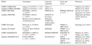
2.1.1 CNRM
Major changes implemented into the atmosphere component of the CNRM-CM5.1 model ARPEGE-Climat version 5 (Voldoire et al., 2013) include in particular updates of the turbulent, convective, and microphysics schemes. The new model CNRM-AM-PRE6 contains a prognostic turbulent kinetic energy (TKE) scheme (Cuxart et al., 2000) that improves the representation of the dry boundary layer while a new unified dry–shallow-deep convection scheme allows for a better transition between convective regimes (Guérémy, 2011; Piriou et al., 2007). The convective scheme solves a prognostic equation for the updraft vertical velocity and uses a convective available potential energy (CAPE) closure. It also features detailed prognostic microphysics (Lopez, 2002), which are consistent with the ones used for large-scale condensation and precipitation. Dust aerosol optical properties have also been updated, as has surface albedo, leading, for instance, to an improved radiation budget in the West African monsoon region (Martin et al., 2017). CNRM-AM6-PRE6 features 91 vertical levels compared to 31 levels in the CMIP5 version.
2.1.2 EC-Earth
The atmosphere model of EC-Earth v2.3 (Hazeleger et al., 2013) has been upgraded from the Integrated Forecasting System (IFS) cy31r1 to IFS cy36r4 and the ocean model to the Nucleus for European Modelling of the Ocean (NEMO) 3.3.1. Major changes in the atmosphere are the new microphysics scheme with six hydrometeor classes, including ice crystals and snow (Forbes et al., 2011), and the new Rapid Radiation Transfer Model (RRTM; Jung et al., 2010). The resolution of the atmosphere model has been increased both horizontally and vertically from T159L62 to T255L91. The ocean component NEMO 3.3.1 is a major upgrade and features a moderate increase in the vertical resolution (from L42 to L46). The sea ice model was upgraded from the Louvain-la-Neuve Sea Ice Model 2 (LIM2) to LIM3 with an improved description of the sea ice rheology and physics. The option of LIM3 to take into account multiple sea ice categories was not used as the Arctic sea ice was found to be unstable in a multi-category setup. Updates of the convection scheme were applied that were developed by the European Centre for Medium-Range Weather Forecasts (ECMWF) and resulted in a better representation of the diurnal cycle of convection (Bechtold et al., 2014).
2.1.3 HadGEM
Changes in the atmospheric component between the HadGEM2 and HadGEM3 model families include the ENDGame dynamical core (Wood et al., 2014), the inclusion of a prognostic cloud and condensate scheme (PC2; Wilson et al., 2008), increased convective entrainment and detrainment, a new orographic gravity wave drag (GWD) representation (Vosper et al., 2009), and numerous other changes (see Walters et al., 2011, 2014, 2017 for details). In addition, the vertical resolution has been increased and the model lid extended from 40 to 85 km. Both of these changes require the model physical schemes to be revisited and adjusted to remove level dependencies and, in some cases, for additional parameterizations to be included, such as the non-orographic GWD scheme (Scaife et al., 2002) to represent momentum deposition by the breaking of gravity waves in the upper stratosphere and mesosphere. The PC2 scheme is a distributed cloud parameterization that represents cloud cover and condensate changes occurring through changes to the environmental temperature and humidity as a result of the other physical parameterizations. In particular, condensate detrained by the convection scheme is handled directly by PC2 rather than being evaporated, detrained, and recondensed as in HadGEM2. Many other changes to the clouds, microphysics, and convection have also been made in order to achieve a reasonable global climatology and radiative balance.
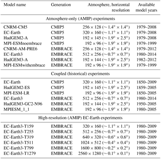
Table 2List of model configurations and model experiments analyzed. If more than one ensemble member is available, only the first ensemble “r1i1p1” is analyzed.
HadGEM3-GC2 (Williams et al., 2015) includes Global Atmosphere 6.0 (Walters et al., 2017), Global Ocean 5.0 (based on NEMO v3.4) with 75 vertical levels, and Global Sea Ice 6.0 (see Table 1). In addition, HadGEM3-GC2 does not include earth system components, such as an interactive carbon cycle, dynamic vegetation, tropospheric chemistry, or ocean biogeochemistry, that are present in the CMIP5 version HadGEM2-ES, but it does include interactive aerosols (with a different tuning for the dust scheme).
2.1.4 MPI-ESM
ECHAM6 and its land component JSBACH have undergone several further developments since the version used for CMIP5 (ECHAM6.1/JSBACH 2.0). Several bug fixes in the physical parameterizations of ECHAM6.3 ensure energy conservation in the total parameterized physics. A recalibration of the cloud processes resulted in a climate sensitivity of about 3 K of the new model system, which is about in the middle of the range of climate sensitivities spanned by the CMIP5 models. JSBACH 3.0 comprises several bug fixes, a new soil carbon model (Goll et al., 2015), and a five-layer soil hydrology scheme (Hagemann and Stacke, 2015) replacing the previous bucket scheme.
2.2 Model experiments
Two kinds of model simulations have been performed: Atmosphere Model Intercomparison Project (AMIP) type simulations, i.e., atmosphere–land only with prescribed SSTs, and coupled CO2 concentration-driven (historical) simulations. AMIP simulations were performed with all four updated models (EC-Earth3, HadGEM3-GA6, which is denoted HadGEM3-A hereafter, CNRM-AM-PRE6, MPI-ESM); the three models EC-Earth3, HadGEM3-GC2, and MPIESM_1_1 were used to perform coupled simulations. For both types of simulations the CMIP5 protocol was followed (Taylor et al., 2012). The model experiments analyzed are summarized in Table 2. The main focus of this study will be on the coupled simulations, as these model configurations are particularly relevant to projecting future climate change.
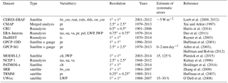
2.3 Observational data
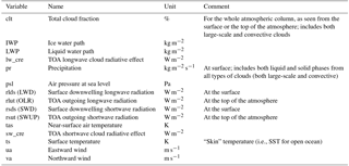
The observational and reanalysis data used for the model evaluation are summarized per dataset in Table 3 and the variable definitions are given in Table 4.
Table 3Observationally based datasets used for the model evaluation. For variable definitions, see Table 4.
3.1 Near-surface temperature and precipitation
Near-surface air temperature and precipitation are controlled by a large number of interacting processes making it challenging to understand and improve model biases in these quantities as model errors can partly compensate for each other. The two variables, however, are frequently analyzed in atmospheric models and can provide an overview and a starting point for further analysis.
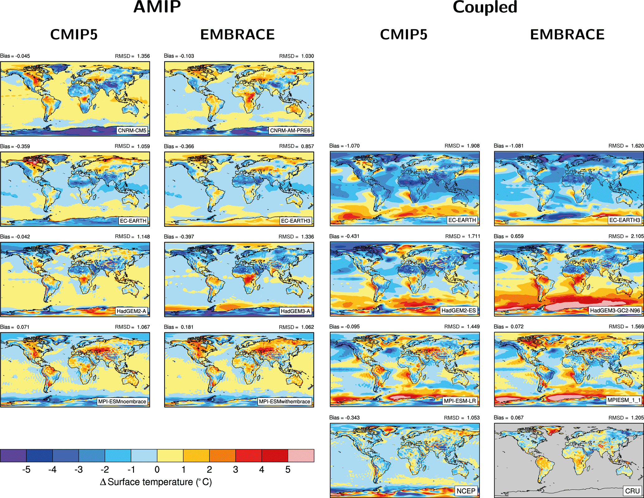
Figure 1Bias in 20-year annual mean near-surface air temperature for the period 1986–2005 (MPI AMIP models: 1980–1999). Shown are the differences between the 20-year climatology from ERA-Interim and the following from left to right: (1) the AMIP simulations from the CMIP5 models, (2) the corresponding EMBRACE models, (3) the coupled historical simulations from the CMIP5 models, and (4) the corresponding EMBRACE models. As alternative reference datasets, data from the NCEP 1 reanalysis and the CRU dataset are shown in the two lowest rightmost panels. The global averaged annual mean bias (“bias”) and root mean square deviation (RMSD) compared with ERA-Interim are given above the individual panels.
3.1.1 Near-surface air temperature
Figure 1 shows the bias in 20-year annual mean near-surface temperatures averaged over the years 1986–2005 from the CMIP5 and EMBRACE models compared with the reanalysis ERA-Interim (Dee et al., 2011). All data have been interpolated to a common 1∘ × 1∘ grid using a bilinear interpolation scheme. The color scale has been adapted from the model evaluation chapter of the Fifth Assessment Report of the Intergovernmental Panel on Climate Change (IPCC-AR5; Flato et al., 2013) to allow for an easy comparison with the CMIP5 multi-model mean bias (their Fig. 9.2b). The mean near-surface temperature from the individual models agrees with the ERA-Interim reanalysis mostly within ±3 ∘C. Larger biases can be seen in regions with sharp gradients in temperature, for example in areas with high topography such as the Himalayas and the sea ice edge in the Southern Ocean.
In the AMIP simulations (left two columns in Fig. 1), the MPI-ESM shows only very modest changes in the simulated mean near-surface temperature bias, whereas particularly EC-Earth3 and CNRM-AM-PRE6 show considerable improvements compared with their CMIP5 versions over North America. The cold biases over large parts of Antarctica found in CNRM-CM5 are also reduced in the EMBRACE version of the model, possibly related to updates in the turbulence scheme and the increased vertical resolution in the lower troposphere. In contrast, the warm bias over Central Africa in CNRM-AM-PRE6 and HadGEM3-A is worse compared with their CMIP5 counterparts and might be partly related to reduced (convective) precipitation in this region (see also Fig. 2) in the EMBRACE versions of the models. In the HadGEM3-A model, the increase in the near-surface temperature bias over India seems to be related to less summer monsoon rainfall (see also Sect. 3.1.2).
In the concentration-driven historical coupled simulations (right two columns in Fig. 1), EC-Earth3 shows a bias reduction over many parts of the continents and over tropical and subtropical oceans, in particular over the Southern Ocean, Central Africa, and northwestern America. Despite these bias reductions, the globally averaged mean bias remains similar at about −1.1 ∘C. This is a consequence of reductions in the warm bias, for example in the Southern Ocean, leading to less error compensation for negative biases in other regions. While the CMIP5 version HadGEM2-ES shows a globally averaged negative bias of about −0.4 ∘C in near-surface temperature, HadGEM3-GC2-N96 has a positive global average bias (∼ 0.7 ∘C). This is particularly caused by larger positive biases over most parts of the Southern Hemisphere ocean and over the tropical areas of Africa and South America in HadGEM3-GC2-N96. In these regions, the near-surface temperature biases in the EMBRACE version are up to 2 ∘C larger than in the predecessor version. Williams et al. (2015) comment that, while both models have a large downwards surface flux bias over the Southern Ocean, the larger coupled SST (and upper ocean heat content) biases appear to be related to changes to both the lateral and vertical ocean heat transports associated with the change in ocean model and ocean resolution. The HadGEM3-GC2 errors also include a contribution associated with too-shallow Southern Ocean summer mixed layers. Model biases in HadGEM3-GC2-N96 are, however, reduced compared with the CMIP5 version, particularly over the American Arctic with bias reductions of about 1 ∘C. The MPI-ESM shows only rather small changes in the simulated annual mean surface temperature between the CMIP5 and EMBRACE version. Similar to the HadGEM3-GC2-N96 model, the warm bias over the Southern Ocean is slightly worse in the EMBRACE simulation than in the CMIP5 simulation.
In the AMIP simulations, biases in the near-surface temperature climatology from the EMBRACE models are particularly reduced in midlatitudes, such as over North America, but are increased in some models over many parts of the tropical continents. In most of the analyzed models, a warm bias over Central Africa and northern South America is still present in the EMBRACE simulations. Particularly in these two tropical regions, however, the observational uncertainties are large as can be seen by comparison of ERA-Interim and the Climate Research Unit (CRU) dataset (Harris et al., 2014) showing differences of up to 2–3 ∘C. Only the temperature bias found in the simulations from the CNRM and HadGEM when compared to ERA-Interim are larger than this estimate of the observational uncertainty in these regions. In the coupled simulations, large biases are still present in the Southern Ocean, in particular along the coast of Antarctica. The coupled EMBRACE models are slightly worse than (HadGEM) or do not systematically outperform (EC-Earth, MPI-ESM) their CMIP5 counterparts in reproducing the ERA-Interim global near-surface temperature distribution in terms of RMSE. Here, it needs to be kept in mind that the EMBRACE models are still prototypes and are not yet fully tuned, which is a particularly challenging and time-consuming task for coupled models.
3.1.2 Total precipitation
Biases commonly found in the simulated mean precipitation from CMIP5 models include too little precipitation along the Equator in the western Pacific associated with ocean–atmosphere feedbacks (Collins et al., 2010) and too-high precipitation amounts in the tropics south of the Equator related to an unrealistic double ITCZ in many models, particularly in the Pacific (Oueslati and Bellon, 2015).
Figure 2 shows the biases in annual mean precipitation averaged over the 20-year period 1986–2005 from the CMIP5 and EMBRACE simulations compared with data from the Global Precipitation Climatology Project (GPCP; Adler et al., 2003). Similarly to Fig. 1, the color scale of Fig. 2 has also been matched with the one used in IPCC-AR5 to allow for an easy comparison with the CMIP5 multi-model mean bias (Flato et al., 2013, their Fig. 9.4b). The model data have been interpolated to the 2.5∘ × 2.5∘ grid of the GPCP observations using a bilinear interpolation scheme. The corresponding relative bias (%) in annual mean precipitation from the models compared with GPCP is shown in Fig. S1 in the Supplement. In contrast to the AMIP simulations with the MPI-ESM showing no large changes in the amplitude and geographical distribution of the precipitation bias between the CMIP5 version (MPI-ESMnoembrace) and the EMBRACE version (MPI-ESMwithembrace), the EMBRACE models CNRM-AM-PRE6, EC-Earth3, and HadGEM3-A show considerable reductions in the precipitation biases compared with their CMIP5 versions. The CNRM-AM-PRE6 AMIP simulation shows a considerable reduction in the wet bias over large parts of the tropical ocean by up to 2 mm day−1 but a slightly worse dry bias in the tropical regions of South America and Africa compared with the CMIP5 simulation from CNRM-CM5. EC-Earth3 also shows a reduction in the wet bias over most parts of the tropical oceans by about 1 mm day−1 and a small reduction in the dry bias over the tropical parts of South America and Africa in comparison to EC-Earth. While the pattern of precipitation biases in HadGEM3-A is similar to that in HadGEM2-A, the magnitude of the bias is reduced in many regions, particularly over the tropical Indian Ocean and western Pacific.
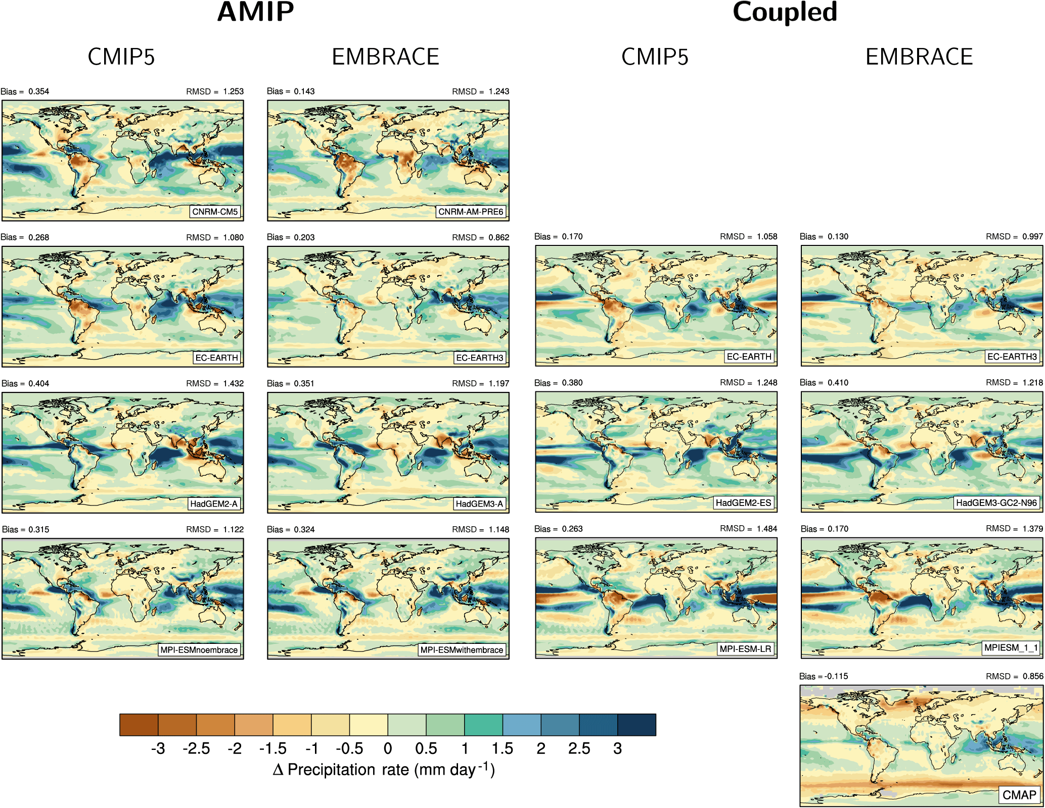
Figure 2Bias in annual mean precipitation rate (mm day−1) for the 20-year period 1986–2005 (MPI AMIP models: 1980–1999) as the difference between the Global Precipitation Climatology Project (GPCP) and from left to right (1) the AMIP simulations from the CMIP5 models, (2) the corresponding EMBRACE models, (3) the coupled historical simulations from the CMIP5 models, and (4) the corresponding EMBRACE models. Data from CMAP are shown as a second reference dataset in the lowermost rightmost panel. The global averaged annual mean bias (“bias”) and root mean square deviation (RMSD) compared with GPCP are given above the individual panels.
In the coupled model simulations (rightmost two columns in Fig. 2), EC-Earth3 shows a similar reduction compared with EC-Earth in the dry bias over northern South America and in the wet bias over the tropical Atlantic to that seen in the AMIP configuration. The differences between the CMIP5 and the EMBRACE simulation from EC-Earth in most other regions are rather small. The coupled simulations with the HadGEM and the MPI-ESM perform quite similarly and do not show large differences between the EMBRACE (HadGEM3-GC2-N96: global average RMSD = 1.22 mm day−1, MPIESM_1_1: RMSD = 1.38 mm day−1) and the CMIP5 versions (HadGEM2-ES: RMSD = 1.25 mm day−1, MPI-ESM-LR: RMSD = 1.48 mm day−1) of the models. On average, the coupled EMBRACE simulation with MPIESM_1_1 results in slightly drier conditions than the one with the CMIP5 model MPI-ESM-LR.
It is noteworthy that the bias reduction in precipitation over tropical oceans with the EMBRACE models is smaller in the coupled experiments than in the atmosphere-only simulations. This is partly due to compensation between precipitation and SST biases in coupled models (e.g., Levine and Turner, 2012; Vanniere et al., 2014). Quantitative assessments are, however, not possible as the model setups of the coupled simulations analyzed here do not exactly match the ones used for the AMIP simulations.
The tropical precipitation in three out of four EMBRACE models analyzed is clearly improved, which can be partly attributed to improved convective precipitation in the models and other updates in the atmospheric components of the model. For example, snow and rain are now prognostic variables in the EMBRACE version of EC-Earth. The wet biases in these regions in the CMIP5 simulations have been reduced by up to 1–2 mm day−1. This reduction in the wet bias of the models also holds when using CMAP data as a reference for comparison (Fig. S2) even though the reduction in absolute bias is smaller as the CMAP data show less precipitation in the tropics and are thus closer to the model results than GPCP.
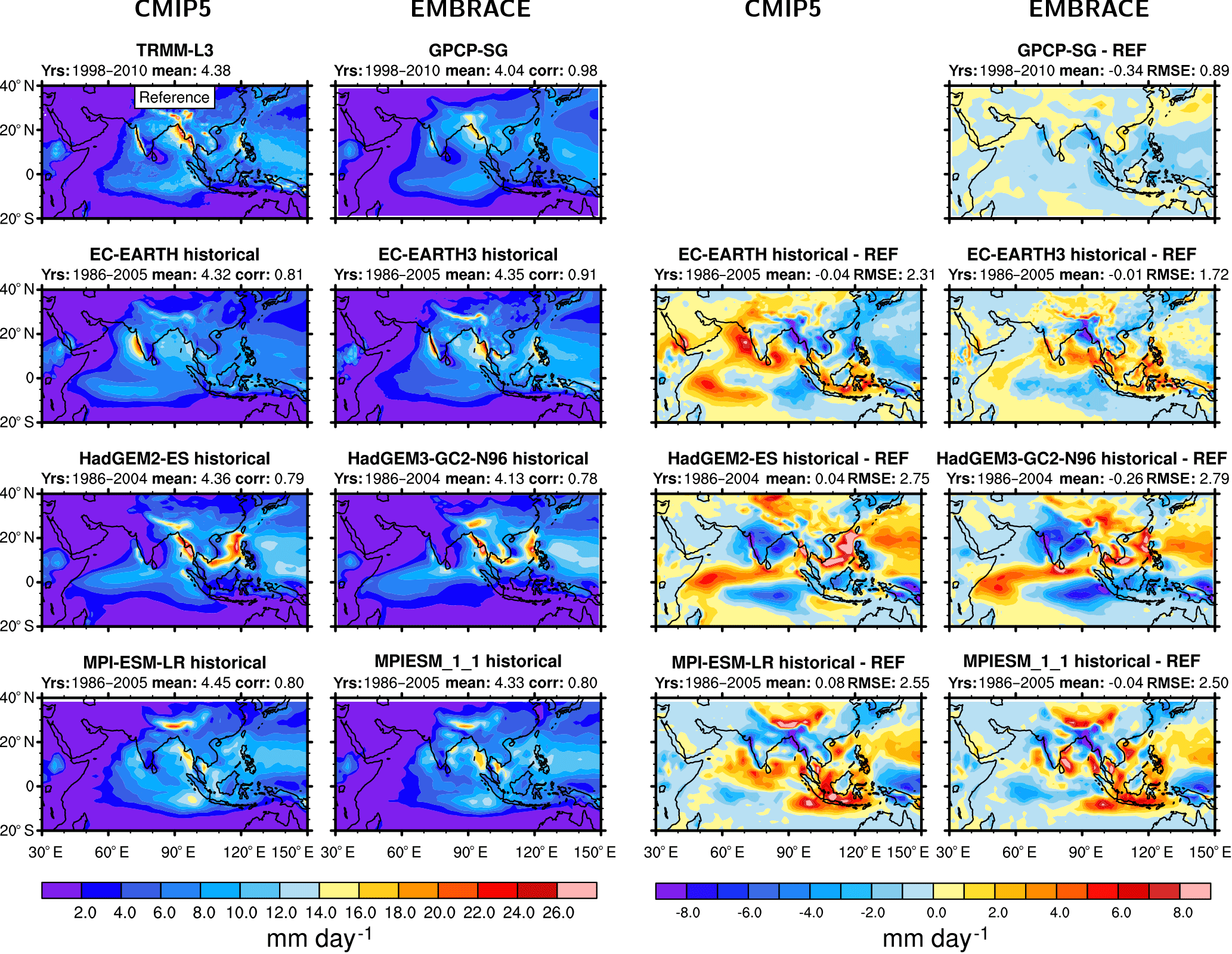
Figure 3Leftmost two columns: seasonal mean precipitation for JJAS from observations (TRMM, GPCP) and the coupled simulations. The years used to calculate the averages shown are given above each panel (“yrs”). Rightmost two columns: differences relative to TRMM. Columns 1 and 3 show the original CMIP5 model versions, columns 2 and 4 the EMBRACE-updated models. The domain-averaged annual mean (“mean”), linear pattern correlation (“corr”; leftmost two columns), mean bias (“mean”), and root mean square error (RMSE; rightmost two columns) compared with TRMM are given above the individual panels.
In the following sections, more regional or process-specific climate phenomena known to exhibit systematic errors in present-day GCMs are evaluated. The following subsections cover (i) the South Asian and West African monsoons, (ii) coupled equatorial oceanic climate, and (iii) Southern Ocean clouds and radiation.
3.2 Monsoon
3.2.1 South Asian monsoon
The South Asian monsoon (referred to as the SAM hereafter) provides over 1 billion people with their primary source of water (Turner and Annamalai, 2012). Reliable estimates of possible future changes in the SAM are therefore crucial for long-term planning in the region (Menon et al., 2013).
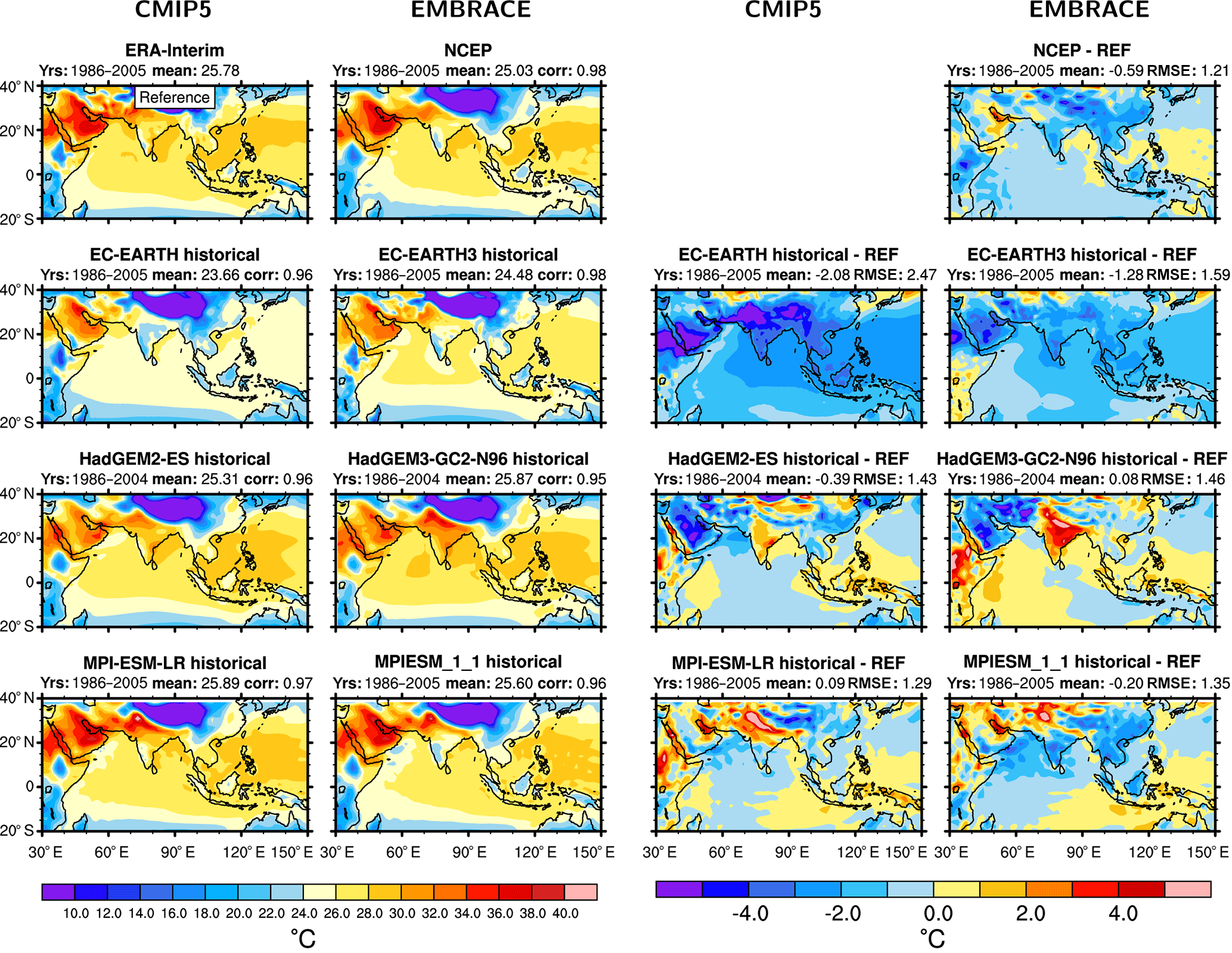
Figure 4Leftmost two columns: seasonal mean 2 m temperature for JJAS from reanalysis data (ERA-Interim), the NCEP 1 dataset, and the coupled simulations averaged over the years 1986–2005 (HadGEM: 1986–2004). Rightmost two columns: differences relative to ERA-Interim. Columns 1 and 3 show the original CMIP5 model versions, columns 2 and 4 the EMBRACE-updated models. The domain-averaged annual mean (“mean”), linear pattern correlation (“corr”; leftmost two columns), mean bias (“mean”), and root mean square error (RMSE; rightmost two columns) compared with ERA-Interim are given above the individual panels.
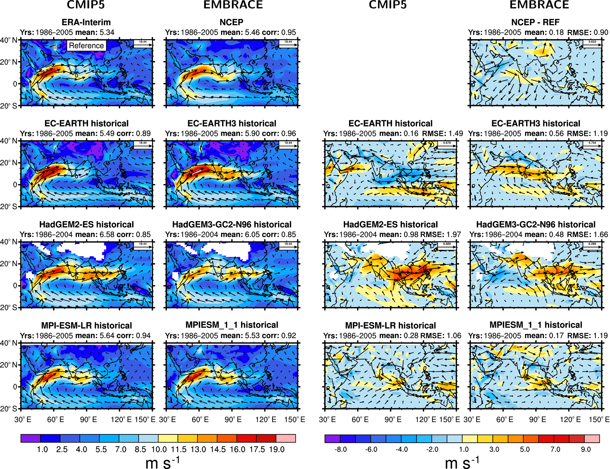
Figure 5Leftmost two columns: seasonal mean zonal wind speed at 850 hPa for JJAS from reanalysis data (ERA-Interim, NCEP 1) and the coupled simulations averaged over the years 1986–2005 (HadGEM: 1986–2004). Rightmost two columns: differences relative to ERA-Interim. Columns 1 and 3 show the original CMIP5 model versions, columns 2 and 4 the EMBRACE-updated models. The domain-averaged annual mean (“mean”), linear pattern correlation (“corr”; leftmost two columns), mean bias (“mean”), and root mean square error (RMSE; rightmost two columns) compared with ERA-Interim are given above the individual panels.
The SAM has two distinct seasonal components. The winter monsoon is dominated by a planetary-scale circulation linked to the Siberian anticyclone and Aleutian low centered over the North Pacific. These features induce northerly flow across South Asia from November to March with minimal amounts of precipitation (Chang et al., 2006). The summer monsoon starts in April, with the onset of rain over southern India and Myanmar generally occurring in early June and propagating northwest, reaching northern India by mid-July. The monsoon rainy season extends to the end of September before reverting back to winter monsoon conditions by November (Chang et al., 2006). Due to the importance of ocean–atmosphere interactions in the evolution of the SAM and because we are primarily interested in evaluating model configurations that can be used for making future projections, here we analyze the ability of the coupled EMBRACE models to represent the main features of the summer SAM. Figure 3 shows seasonal mean (June to September, JJAS) precipitation from the coupled models and the differences relative to the satellite product TRMM 3BV43 (Huffman et al., 2007). Figures 4 and 5 show near-surface temperature and 850 hPa zonal wind speed compared to data from the ERA-Interim reanalysis. Also shown are the alternative observation-based datasets GPCP-SG (precipitation) and the NCEP 1 reanalysis (Kalnay et al., 1996; near-surface temperature and zonal wind speed).
In the observations, a precipitation maximum is seen on the western coast of India, with a relative minimum on the lee side of the Western Ghats. Further maxima are seen along the coast of Myanmar and Laos (eastern coast of the Bay of Bengal) and along the foothills of the Himalayas. A broad region of precipitation is also evident in central and northeastern India. EC-Earth and MPI-ESM capture these primary rainfall features with varying degrees of accuracy. EC-Earth overestimates rainfall over the ocean adjacent to the Western Ghats and over the Bay of Bengal. Farther east, over Myanmar and Laos, precipitation is underestimated. The positive precipitation bias over the ocean is clearly improved in EC-Earth3. Both MPI-ESM versions underestimate rainfall over the Indian subcontinent, with particular negative biases associated with the Western Ghats mountains and the foothills of the Himalayas likely caused by the low resolution of MPI-ESM. There is little difference between the two MPI-ESM configurations. The major precipitation biases are also largely unchanged between the two HadGEMs, with an underestimate of precipitation across India and a secondary negative bias south of India along the Equator. The process of irrigation that is missing in current GCMs might contribute to the dry bias over northern India. Saeed et al. (2009) found that temperature biases caused by a too-strong differential heating between land and sea if no irrigation is considered can lead to unrealistic simulations of the SAM circulation and associated rainfall in climate models.
The HadGEMs (particularly HadGEM3-GC2) show a large warm bias in 2 m temperature over the Indian land mass (Fig. 4). This error is linked to excess downwelling surface shortwave radiation (of up to 60 W m−2 in the JJAS mean) due to a lack of optically thick clouds over India. The lack of simulated rainfall exacerbates this problem further, leading to a dry land-surface bias, reduced surface evaporative cooling, and increased surface sensible heat flux. The converse is seen in both EC-Earth coupled simulations, with a cold bias of ∼ 5 ∘C over India linked to an underestimate of downwelling solar radiation of ∼ 40 W m−2. The domain-averaged cold bias in the EMBRACE simulation with EC-Earth is, however, considerably reduced from −2.1 ∘C in the CMIP5 version of the model to −1.3 ∘C in the EMBRACE version.
All of the models represent the cross-equatorial low-level jet and acceleration of the westerly monsoon flow across the Arabian Sea (Fig. 5), though the strength of the jet core and the eastward extension of the westerlies towards the Philippines vary between models. Positive biases in 850 hPa wind speed are reduced in the HadGEM3-GC2-N96 model and are replaced by a negative bias over the Arabian Sea. In contrast, the largely negative biases in EC-Earth are replaced by a positive bias in EC-Earth3. Both EC-Earth configurations, and to a lesser extent the MPI-ESMs and HadGEM3-ES, have a cold SST bias across the western Indian Ocean and Arabian Sea (as seen from the biases in 2 m temperature in Fig. 4). For a given low-level wind speed a cold bias in Arabian Sea SSTs will act to decrease surface ocean evaporation (relative to the correct SST) and thus reduce the atmospheric moisture flux into India and consequently precipitation, while a cold bias in the equatorial Indian Ocean contributes to the meridional temperature gradient and thereby enhances the monsoon flow (Levine and Turner, 2012; Levine et al., 2013).
In particular, the performance in terms of the averaged RMSE of EC-Earth3 for the variables precipitation, near-surface temperature, and 850 hPa zonal wind speed is improved compared to its CMIP5 predecessor (see EC-Earth panels in Figs. 3–5). For HadGEM3, the domain-averaged bias in RMSE for 850 hPa zonal wind speed is reduced from 1.97 to 1.66 ms−1 compared to HadGEM2. In contrast, 2 m temperature and precipitation patterns from HadGEM3 show improvements in some regions but degradation in agreement with ERA-Interim in other regions such as India. This kind of performance degradation seen in some regions is probably at least partly related to these being prototype model configurations and thus may or may not improve in the final model versions. The changes in the MPI-ESM configuration do not show a large impact on the simulated WAM, resulting in a rather similar performance of the CMIP5 and the EMBRACE version of MPI-ESM.
Figure 6 summarizes the annual cycle of SAM, sampling both precipitation and dynamical measures. Figure 6a shows the mean annual cycle of precipitation spatially averaged over 5 to 30∘ N and 65 to 95∘ E. EC-Earth overestimates both the duration of the monsoon rainy season and the mean rainfall intensity during the peak monsoon. Both these biases are improved in EC-Earth3. There is little difference between the two MPI-ESMs, which at this spatial scale exhibit an accurate simulation of monsoon rainfall. The two HadGEM configurations underestimate rainfall, with biases particularly large in the early monsoon period (May to July). Through bias compensation, the multi-model mean provides the most accurate mean annual cycle. Figure 6b shows the annual cycle of the Webster and Yang (1992; hereafter WY) dynamical monsoon index and Fig. 6c the Goswami index (Goswami et al., 1999, hereafter GM). The WY index is based on vertical shear of the tropospheric zonal wind speed (u850 hpa − u200 hpa) averaged over 40–110∘ E and 0–20∘ N, while the GM index is a measure of the vertical shear in the meridional wind speed (v850 hpa − v200 hpa) averaged over 70–110∘ E and 10–30∘ N. Both capture the interplay between large-scale dynamics and atmospheric diabatic heating over the Indian region. The WY index is a measure of the large-scale southwesterly monsoon circulation, while the GM index is a measure of the Hadley circulation intensity and meridional propagation. All models exhibit considerably more accuracy in simulating these dynamical measures compared to SAM precipitation, particularly the WY index, although part of this improved performance stems from error compensation between lower tropospheric (850 hPa) and upper tropospheric (200 hPa) wind speed biases (not shown).
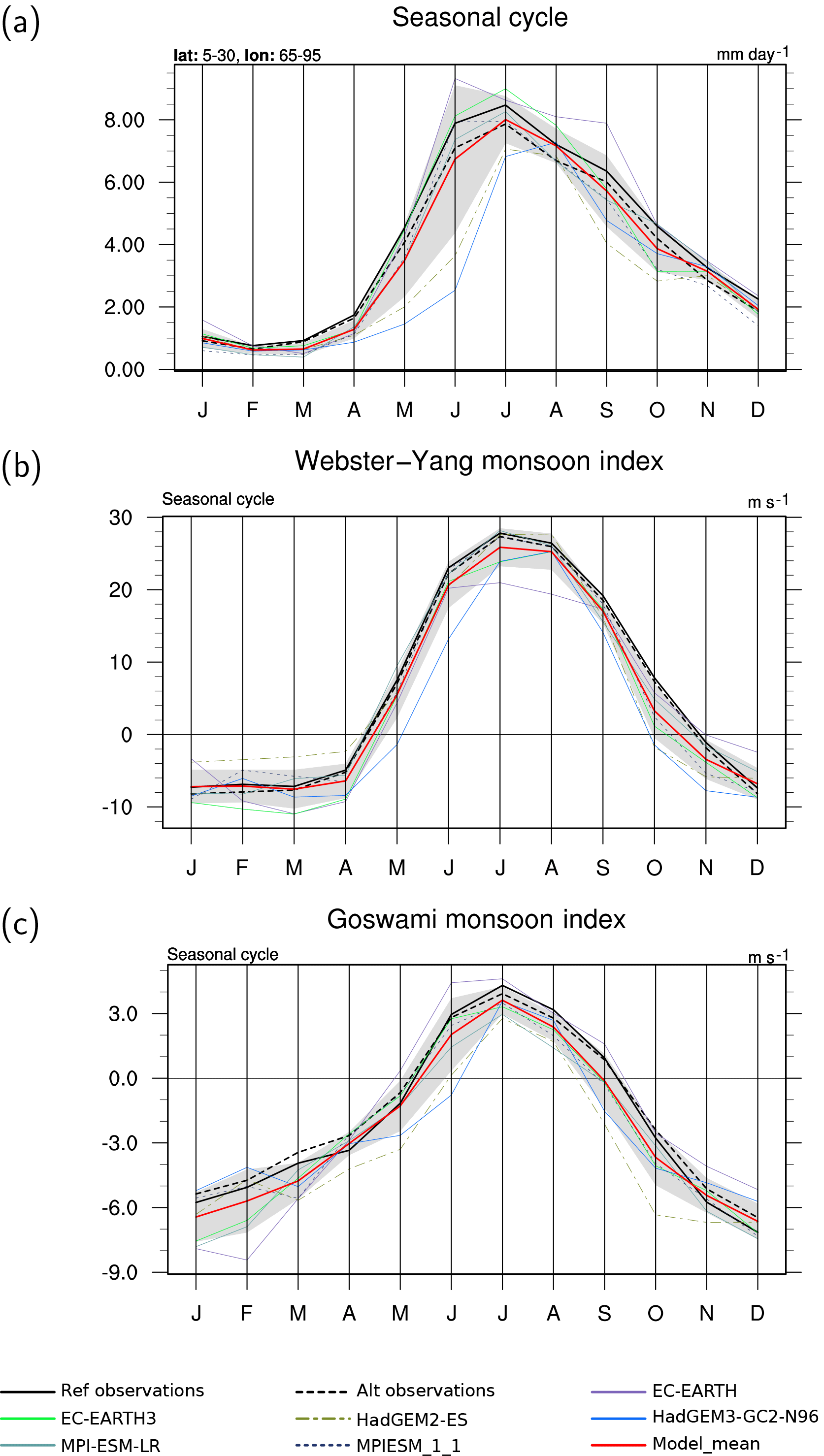
Figure 6Mean annual cycle plots averaged over the years 1986–2005 (HadGEM: 1986–2004): (a) precipitation spatially averaged over 5–30∘ N, 65–95∘ E, (b) Webster and Yang monsoon index, (c) Goswami monsoon index. Shown are the coupled (historical) simulations. The reference observations (a) TRMM-L3 and (b, c) ERA-Interim are shown as solid black lines, the alternative observations (a) GPCP-SG and (b, c) NCEP 1 as black dashed lines.
All of the EMBRACE coupled models exhibit considerable biases with respect to monsoon precipitation. Only EC-Earth3 showed a measurable improvement over its CMIP5 predecessor. Most of the models appear to capture the large-scale dynamical evolution of the SAM, but fail to capture the associated evolution of precipitation, particularly the sub-continental distribution of rainfall, although on the scale of “all India” the MPI-ESMs do capture the annual cycle quite well. Models continue to have severe problems capturing the subtle interactions between deep convection, cloud–radiation processes, precipitation, and surface evaporation with the associated interplay between diabatic heating over land and the large-scale monsoon circulation with the associated oceanic evaporation.
3.2.2 West African monsoon
West Africa also experiences a summer monsoon from May to October (Nicholson and Grist, 2003) with rains starting in May at the Guinea coast and propagating northward to the Sahel region (∼ 15∘ N) by mid-July (Sultan and Janicot, 2003). Failures in the West African monsoon (hereafter WAM) or lack of northward propagation into the Sahel can have devastating consequences for the population of this region, as evidenced by the extensive famines during the 1970s and 1980s linked to decadal variability in WAM rainfall (Held et al., 2005; Nicholson et al., 2000). As with the SAM, the WAM also results from the seasonal development of a low-level thermal gradient between the tropical ocean and the Sahara (Caniaux et al., 2011; Lavaysse et al., 2009). This monsoon circulation and the associated low-level moisture flow interact with westward-propagating, synoptic-scale African easterly waves (AEWs; Poan et al., 2013, 2015) that grow on the southern and northern flanks of the African easterly jet (Thorncroft and Hoskins, 1994a, b; hereafter AEJ). This interaction between AEWs and the monsoon moisture flux supports the development of organized mesoscale convective systems (MCSs) embedded within the AEWs. These MCSs deliver the majority of rainfall over West Africa (Fink and Reiner, 2003; Mathon et al., 2002). Such interaction across scales (mesoscale, convective, synoptic, and planetary scales) is at the heart of WAM dynamics and is a challenge for GCMs, which prevents them from accurately simulating this system, including both natural variability and a forced response to increased greenhouse gases driving precipitation changes (Biasutti, 2013; Roehrig et al., 2013; Ruti and Dell'Aquila, 2010).
Figures 7 and 8 show absolute values of JJAS mean precipitation and 2 m temperature as well as their biases over West Africa compared with observations from TRMM and ERA-Interim reanalysis data, respectively. Differences between TRMM and GPCP for precipitation and ERA-Interim versus Climatic Research Unit (CRU; Harris et al., 2014) data for 2 m temperature give an estimate of observational uncertainty in the region. The WAM is marked by a maximum in precipitation stretching from the Atlantic coast across to the Darfur mountains in Sudan over a latitude band ∼ 5 to 15∘ N. Directly north of the precipitation maximum, near-surface temperatures increase rapidly over the Sahara. Surface warming induces a deep near-surface low-pressure system (the Saharan heat low, Lavaysse et al., 2009) that is one of the main drivers of the low-level southwesterly flow into West Africa.
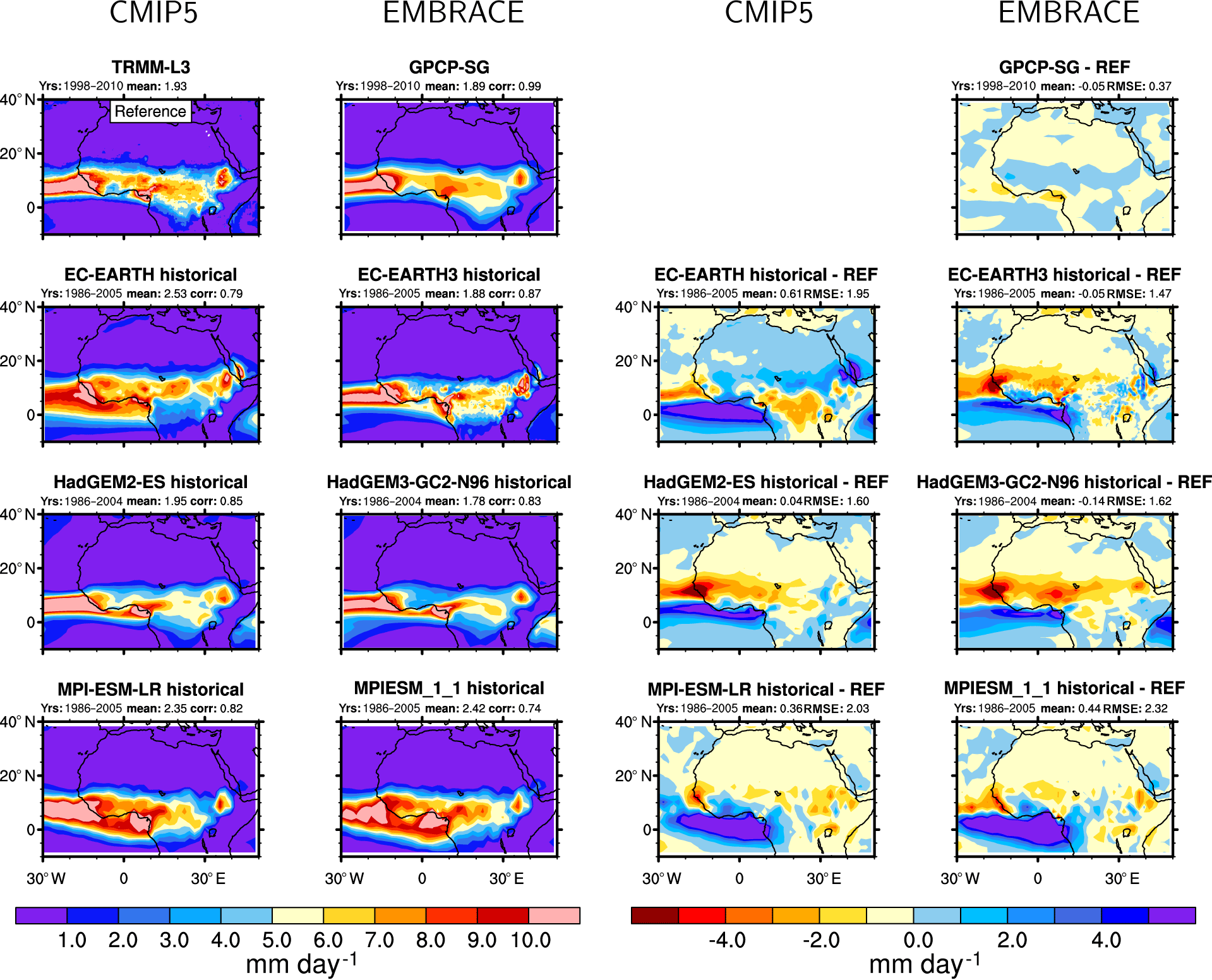
Figure 7Leftmost two columns: seasonal mean precipitation for JJAS from observations (TRMM, GPCP) and the coupled simulations. The years used to calculate the averages shown are given above each panel (“yrs”). Rightmost two columns: differences relative to TRMM. Columns 1 and 3 show the original CMIP5 model versions, columns 2 and 4 the EMBRACE-updated models. The domain-averaged annual mean (“mean”), linear pattern correlation (“corr”; leftmost two columns), mean bias (“mean”), and root mean square error (RMSE; rightmost two columns) compared with TRMM are given above the individual panels.
All the coupled models exhibit a positive precipitation bias over the Gulf of Guinea. This error is reduced when the models are run with prescribe SSTs (not shown). Such precipitation errors are associated with a warm bias in all three models' SST fields off the coast of Namibia and Angola (evident in the 2 m temperatures; Fig. 8). The warm SST bias, in combination with the predominant southerly low-level atmospheric flow into West Africa (Fig. 9), drives a large (and excessive) low-level moisture convergence into the Guinea coast region and is arguably the main cause of the precipitation bias. Positive SST biases in this region are common to coupled GCMs (Toniazzo and Woolnough, 2014) and are thought to arise from a combination of poorly resolved coastal ocean dynamics (Wahl et al., 2011; Xu et al., 2014), atmospheric wind forcing (Richter and Xie, 2008; Voldoire et al., 2014), and poor simulation of marine stratocumulus clouds (Huang et al., 2007). EC-Earth3 has somewhat improved SST biases in this region compared to its CMIP5 version, which may partly explain the reduced rainfall bias off the Guinea coast.
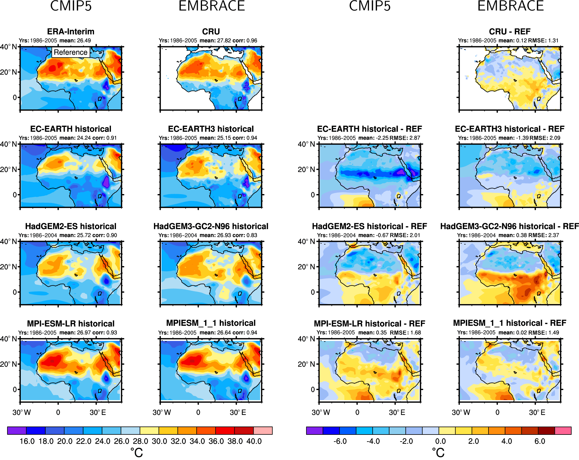
Figure 8Leftmost two columns: seasonal mean 2 m temperature for JJAS from reanalysis data (ERA-Interim), the CRU dataset, and the coupled simulations averaged over the years 1986–2005 (HadGEM: 1986–2004). Rightmost two columns: differences relative to ERA-Interim. Columns 1 and 3 show the original CMIP5 model versions, columns 2 and 4 the EMBRACE-updated models. The domain-averaged annual mean (“mean”), linear pattern correlation (“corr”; leftmost two columns), mean bias (“mean”), and root mean square error (RMSE; rightmost two columns) compared with ERA-Interim are given above the individual panels.
Figure 9 shows the 925 hPa wind velocity over West Africa. Strong southwesterly flow is evident from the Gulf of Guinea into West Africa. EC-Earth and both MPI-ESMs have a large westerly (zonal) bias in the low-level flow suggestive of convergence driven by convective heating of the atmosphere over the Gulf of Guinea. These three models also show the largest positive bias in precipitation in this region. This bias is particularly marked for the EMBRACE version of the MPI-ESM. EC-Earth3 has an improved low-level wind structure compared to EC-Earth, likely due to a combination of improved SST off Angola, reduced convection over the Gulf of Guinea, and a reduction of the cold bias in 2 m temperatures (Fig. 8). Both HadGEMs indicate southwesterly flow into West Africa but a negative (northerly) wind bias north of ∼ 15∘ N indicative of the WAM not penetrating sufficiently far north through the summer season.
Similarly to the analysis of the SAM, EC-Earth3 shows an improvement in the averaged RMSE values for precipitation, 2 m temperature, and 925 hPa zonal wind speed in the WAM region compared to its CMIP5 version (see numbers above EC-Earth panels in Figs. 7–9). For the MPI-ESMs and the HadGEMs, some regional improvements in these variables are partly compensated for by performance degradation in other regions, resulting in similar or slightly worse domain-averaged RMSE values.
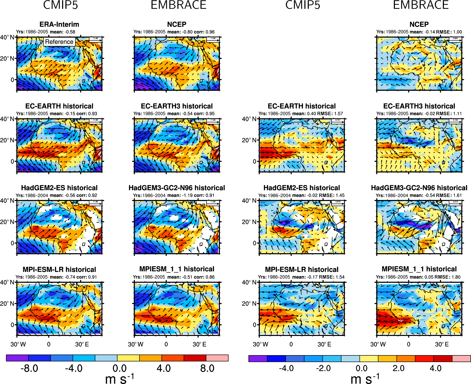
Figure 9Leftmost two columns: seasonal mean wind speed at 925 hPa for JJAS from reanalysis data (ERA-Interim and NCEP 1) and the coupled simulations averaged over the years 1986–2005 (HadGEM: 1986–2004). Rightmost two columns: differences relative to ERA-Interim. Columns 1 and 3 show the original CMIP5 model versions, columns 2 and 4 the EMBRACE-updated models. The domain-averaged annual mean (“mean”), linear pattern correlation (“corr”; leftmost two columns), mean bias (“mean”), and root mean square error (RMSE; rightmost two columns) compared with ERA-Interim are given above the individual panels.
Latitudinal cross sections of precipitation, 2 m temperature, and key radiation variables averaged from 10∘ W to 10∘ E for the JJAS season are shown in Fig. 10. A maximum in 2 m temperatures (Fig. 10a) coincides with a minimum in sea level pressure (Fig. 10b) associated with the Saharan heat low (around 22∘ N). While there is some discrepancy between the simulated 2 m temperature and the two observationally based datasets (ERA-Interim and CRU), all models capture the sharp increase in temperature around 15∘ N although maximum temperatures over the Sahara can vary by 5 ∘C across models. Most models also capture the location and intensity of the Saharan heat low fairly well. Surprisingly, the warmest model over the Sahara (MPI-ESM) has the weakest low-pressure minimum and HadGEM3-GC2, with one of the deepest low pressures, has relatively cool temperatures over the Sahara. Possibly more significant, the location of the low-pressure minimum in HadGEM3-GC2 is displaced ∼ 500 km south of the observed minimum. A key driver of high Saharan surface temperatures is surface absorption of solar radiation. Figure 10c shows downwelling surface solar radiation (SWD) with CERES-EBAF satellite-derived estimates as an observationally based reference (Loeb et al., 2009). A relative minimum in SWD around 10∘ N coincides with the main band of precipitation (Fig. 10g) and associated optically thick clouds. Farther north SWD increases to 300 W m−2 at 25∘ N. Model SWD shows a wide spread over the Sahara ranging from 280 W m−2 in MPI-ESM to 330 W m−2 in the two HadGEM simulations. While the HadGEMs have the highest incoming SWD values over the Sahara, they simulate one of the coldest Saharan 2 m temperatures. This discrepancy most likely arises from a positive surface albedo bias over the Sahara in the HadGEMs. The probable cause of the variable SWD across models is either erroneous optically thin ice clouds and/or a poor representation of Saharan dust, other aerosols, and their interaction with solar radiation. MPI-ESM and EC-Earth3 have relatively accurate representations of both SWD and 2 m temperature over the Sahara. Surface temperatures are considerably improved moving from EC-Earth to EC-Earth3. Downwelling surface longwave radiation (LWD; Fig. 10d) is underestimated by all models over the Sahara except the MPI-ESMs.
Figure 10e shows a cross section of the shortwave (SW) cloud radiative effect (CRE) for JJAS. Negative SW CRE indicates that clouds reduce the amount of SW radiation absorbed by the atmosphere–surface system relative to an equivalent clear-sky atmosphere (i.e., increased SW reflection). This is clearly visible around 10∘ N where CERES indicates a reduction in absorbed SW of −90 W m−2 due to clouds. Cloud effects drop to −10 W m−2 over the Sahara. Both HadGEMs simulate SW CRE over the Sahara close to 0 W m−2, indicative of zero cloud cover. This may partly explain the high bias in SWD seen in HadGEM. The longwave cloud radiative effect (LW CRE) is shown in Fig. 10f, with positive values indicating that clouds reduce the amount of outgoing longwave radiation (OLR) relative to a clear-sky equivalent atmosphere (i.e., more terrestrially emitted radiation trapped in the atmosphere). The precipitation cloud maximum at 10∘ N is delineated by a maximum in LW CRE of 40 W m−2. The majority of models underestimate LW CRE compared to CERES, particularly in the latitude band 10–20∘ N. In this band most models also underestimate the negative cloud radiative effect SW CRE, indicating that model clouds in this band are optically too thin, which is consistent with an underestimate of rainfall in this band in most models.
Zonally averaged precipitation between 10∘ W and 10∘ E from TRMM-3B43 and GPCP-1DD show relatively good agreement (Fig. 10g). The majority of models fail to represent the rapid increase in precipitation between 0 and 5∘ N close to the Guinea coast due to excessive precipitation over the ocean. Most models represent the second maximum in precipitation around 12∘ N, linked to AEWs on the southern flank of the African easterly jet. HadGEM, EC-Earth, and MPI-ESM are all somewhat deficient in rainfall, particularly in the northern maxima region, which is consistent with the cloud–radiation errors discussed above. There is no clear improvement in precipitation between the CMIP5 models and the EMBRACE-updated models.
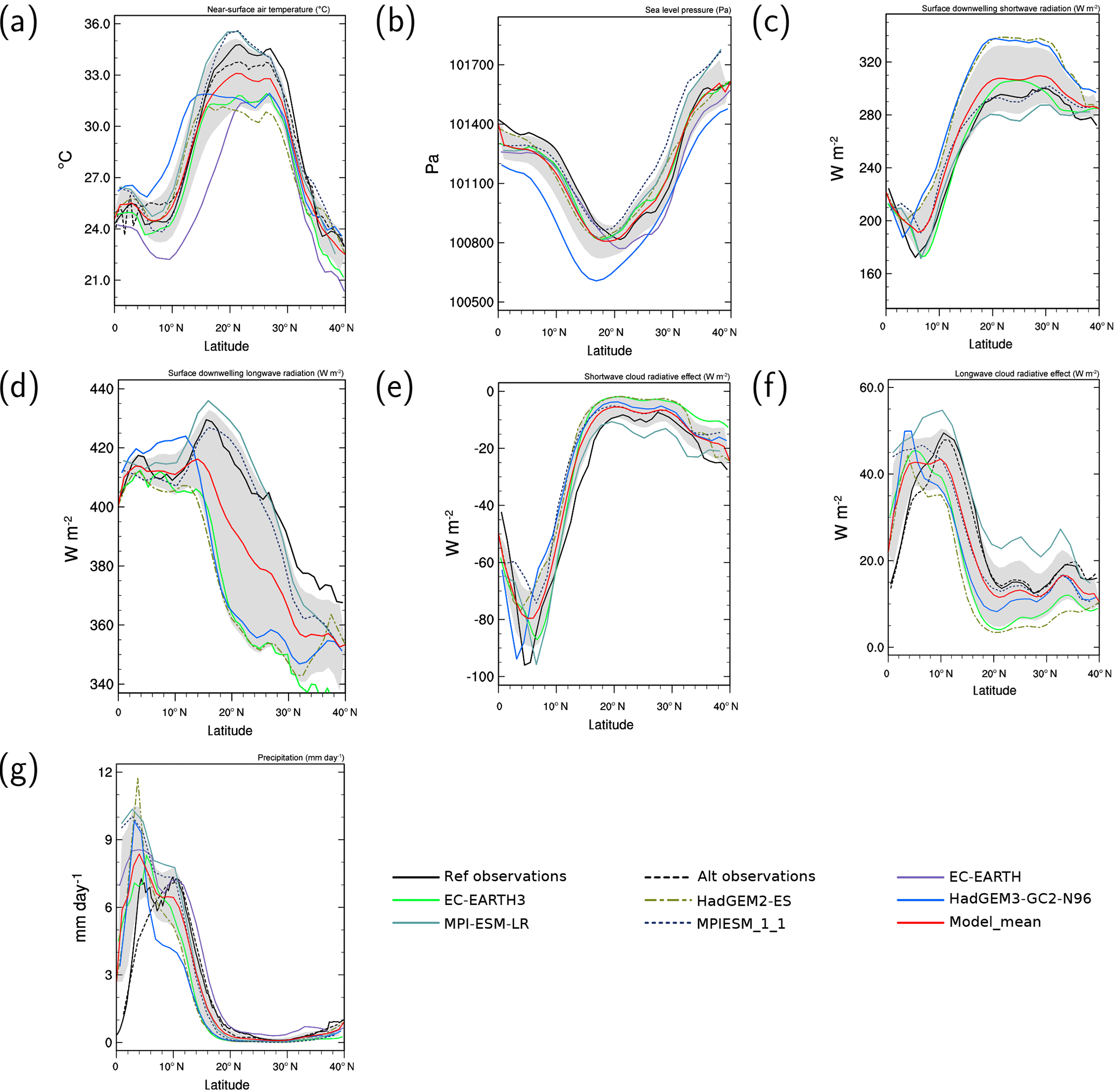
Figure 10The 10∘ W–10∘ E zonal average JJAS mean values averaged over the years 1986–2005 (HadGEM: 1986–2004) as a function of latitude (x axis) for (a) 2 m temperature, (b) sea level pressure, (c) surface downwelling solar radiation, (d) surface downwelling longwave radiation, (e) shortwave cloud radiative forcing, (f) longwave cloud radiative forcing, and (g) precipitation. Model results are for the coupled simulations. The reference observations (a, b) ERA-Interim, (c–f) CERES-EBAF, and (g) TRMM-L3 are shown as solid black lines, the alternative observations (a) CRU, (f) SRB, and (g) GPCP-SG as black dashed lines. The gray shading shows the inter-model standard deviation.
In addition to simulating seasonal mean statistics of the WAM and SAM, it is important that models also represent the underlying weather variability that makes up the seasonal mean precipitation. Any future changes in intra-seasonal precipitation variability will likely have as big an impact on societies in the two regions as changes in seasonal mean monsoon rainfall. The 3–10-day band-pass-filtered variance in precipitation (Fig. 11) emphasizes the dominant timescale of precipitation variability over West Africa. This variability is associated with westward-propagating AEWs and MCSs embedded within these waves. Both TRMM and GPCP show large variance in precipitation on these timescales, stretching from the Darfur mountains west across the Sahel region, with maximum values westward from ∼ 0∘ E to the Atlantic coast coincident with the southern flank of the AEJ.
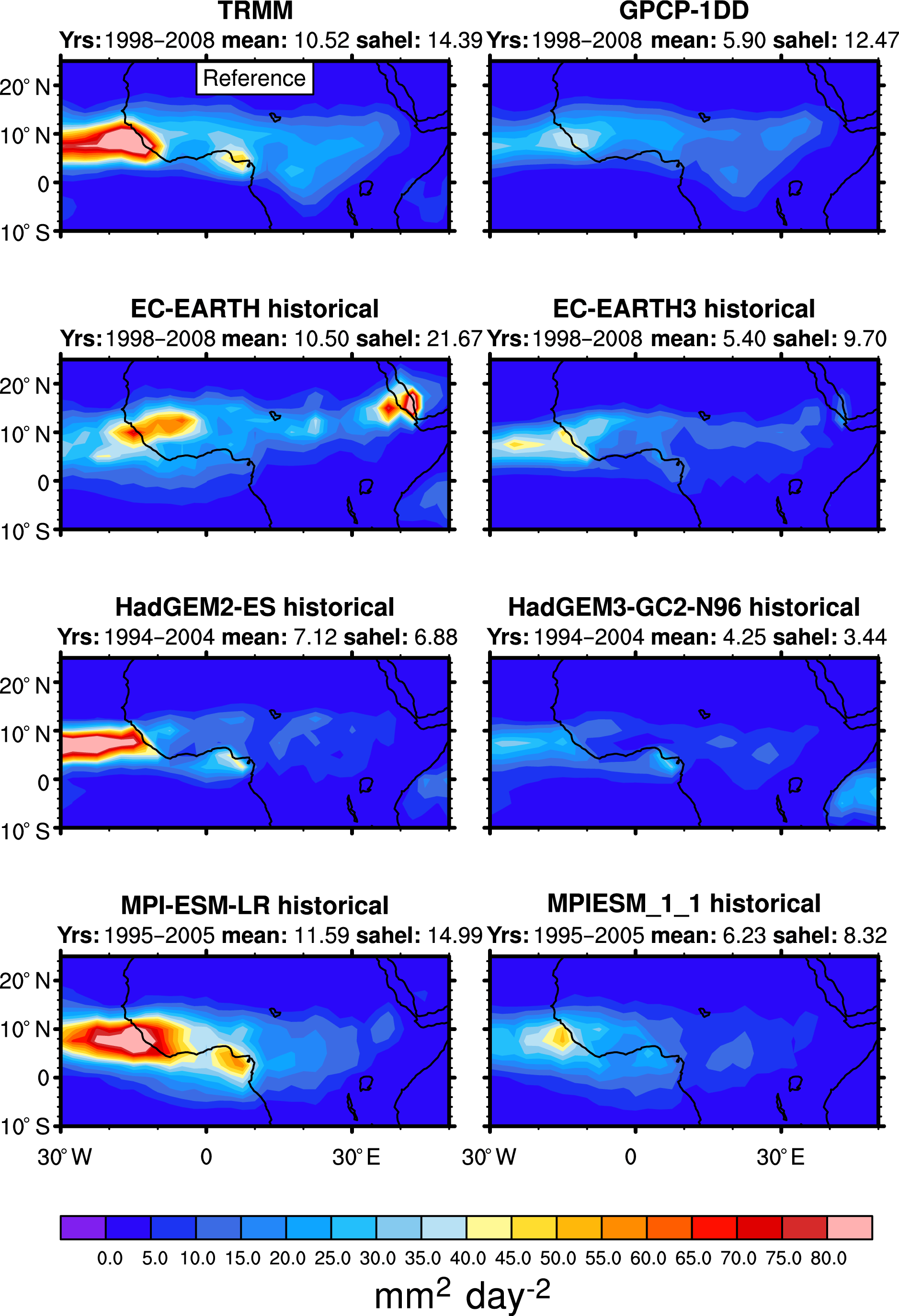
Figure 11JJAS average 3–10-day band-pass-filtered precipitation variance (mm2 day−2) calculated from 11 years of daily precipitation fields as indicated above the panels. The top two panels show observations from TRMM (left panels) and GPCP-1DD (right panels). Shown are the coupled simulations from (left panels) the CMIP5 and (right panels) the EMBRACE-updated models. All data have been interpolated onto a common 2.5∘ × 2.5∘ grid. The band-pass-filtered precipitation variances averaged over the whole domain (“mean”) and over the rectangular region 10∘ W–10∘ E, 10–20∘ N (“sahel”) are given above the individual panels.
Despite the relatively similar time mean (climatological) precipitation from TRMM and GPCP-1DD, the precipitation variabilities from TRMM and GPCP-1DD show large differences. As the base TRMM observational data are at 0.25∘ of spatial resolution and 3-hourly temporal resolution, whereas the GPCP-1DD data are at a spatial resolution of 1∘ and the highest temporal resolution is daily mean values, we would expect TRMM to sample the high temporal and spatial variability in convective precipitation in this region more accurately than GPCP-1DD. In this analysis, we therefore use TRMM as our main reference dataset. EC-Earth appears to capture the northern band of precipitation variability quite well, although this is degraded in EC-Earth3 west of the 0∘ meridian. Both the HadGEMs and MPI-ESMs fail to capture sufficient precipitation variability on these timescales over land compared with TRMM, with significant variability only occurring over the tropical ocean regions. All three coupled EMBRACE models show less precipitation variability than their CMIP5 counterparts. Such findings emphasize the need for an improved representation of wave–precipitation interactions in all coupled models before they can provide robust estimates of changes in intra-seasonal rainfall over this region.
Higher model resolution is generally considered an important route for improving weather timescale variability in climate models (Jung et al., 2012; Roberts et al., 2015). In the following section we present an analysis of EC-Earth simulations run with prescribed SSTs (AMIP mode) sampling horizontal resolutions from T159 (125 km) to T1279 (16 km). In this analysis we focus on the potential benefit that increased atmospheric model resolution brings to simulating synoptic (weather) timescale precipitation variability over both the WAM and SAM regions. Presently these findings are for one EMBRACE model only, but are likely pertinent to model development priorities across modeling groups.

Figure 12The 3–10-day band-pass-filtered JJAS precipitation variance for TRMM (0.25∘ × 0.25∘), GPCP-1DD (1∘ × 1∘), and T159, T255, T319, T511, T799, and T1279 EC-Earth simulations (mm2 day−2).
3.2.3 Representing synoptic timescale precipitation variability in monsoon systems: the role of increased model resolution
While an accurate representation of the mean monsoon climatology, in particular the annual cycle, is a fundamental requirement of GCMs, rainfall variability within the monsoon season is also of importance to the predominantly agrarian societies of West Africa and South Asia. Over the Sahel, the majority of precipitation occurs from intermittent mesoscale convective complexes (MCSs) embedded within westward-propagating synoptic African easterly waves (Mathon et al., 2002), with a clear peak in precipitation variability on the 2–8-day timescale (Kiladis et al., 2006). Similarly over the SAM region, a significant amount of rainfall is associated with synoptic-scale monsoon depressions that develop over the Bay of Bengal before propagating northwestward across India and eventually dissipating over northwestern India or Pakistan (Hunt et al., 2016). To assess the ability of GCMs to accurately simulate this synoptic rainfall we follow the approach described in the previous section and apply a 3–10-day band-pass filter to model and observed precipitation to highlight variability on the timescales of interest.
It is becoming increasingly established that higher model resolution provides a more realistic representation of the underpinning processes controlling weather and precipitation variability (e.g., Dawson and Palmer, 2015; Demory et al., 2014; Jung et al., 2012). In order to assess the benefit that higher model resolution brings to the simulation of sub-seasonal precipitation variability over the WAM and SAM, in this section we analyze one of the EMBRACE models (EC-Earth) run in AMIP mode for the period 1980–2009, sampling atmospheric model horizontal resolutions of T159 (128 km), T255 (80 km), T319 (64 km), T511 (40 km), T799 (25 km), and T1279 (16 km) with a common set of 91 vertical levels. The findings from this analysis may offer pointers for an optimal resolution for other models to aim at with respect to simulating sub-seasonal precipitation variability and seasonal mean rainfall.

Figure 13The 3–10 day band-pass-filtered JJAS precipitation variance for TRMM (0.25∘ × 0.25∘), GPCP-1DD (1∘ × 1∘), and the T159, T255, T319, T511, T799, and T1279 EC-Earth simulations (mm2 day−2).
Figure 12 shows 3–10-day band-pass-filtered precipitation variance for JJAS over Africa from two observational datasets (TRMM 3B42 and GPCP-1DD) and the six EC-Earth resolutions. The two observations differ markedly with respect to the absolute magnitude of variance on these timescales. This is partly expected as the observational datasets feature a rather different horizontal resolution (0.25∘ vs. 1∘). They do, however, exhibit some agreement in the spatial distribution of maxima and minima in precipitation variability, with a broad region of high variability stretching from Sudan west across to the Atlantic coast. GPCP-1DD indicates a northerly maximum in variability over West Africa around 12∘ N associated with AEWs growing on the northern flank of the AEJ. Both datasets indicate a maximum in variability at the Atlantic coast around 10∘ N and relative maxima over the Ethiopian Highlands and Darfur mountains. In EC-Earth, precipitation variability increases (and improves compared to the observations) as model resolution increases from T159 to T511. Beyond T511 there is little further increase in variability. In particular, as resolution increases from T159 to T511, higher variability appears eastwards back across the AEW wave track towards Ethiopia. There is also a clear increase in variability (wave activity and intensity) at the Atlantic coast. Perhaps surprisingly, this increase in precipitation variability is not seen in the 850 hPa meridional wind variability (not shown), which is a typical measure of the AEW activity. Meridional wind variability is well simulated at T159 resolution and largely does not change up to T1279. Hence, the increased model resolution seems to directly impact moist processes that lead to rainfall on the ground, while having only minimal impact on the dynamical structure of the AEWs. It is also worth noting that the seasonal mean (JJAS) precipitation changes very little across the EC-Earth resolutions (not shown), suggesting that at lower resolutions (below T319), seasonal mean precipitation in EC-Earth, while relatively accurate, is made up of incorrect higher-time-frequency (weather) variability and intensities.
Figure 13 shows 3–10-day filtered JJAS precipitation variance over the extended SAM region, and again both TRMM and GPCP-1DD observations are plotted. As over the WAM region, variability is significantly higher in TRMM than GPCP with this being particularly the case over the equatorial Indian Ocean. Also similar to the WAM, precipitation variability increases (and improves) in EC-Earth as model resolution increases from T159 to T511, with little change thereafter. This increase is true for variability associated with the SAM itself but is not the case for variability over the equatorial Indian Ocean, which in fact slightly decreases (and degrades) as resolution increases beyond T255. As with the WAM, there is only a slight change (an increase) in seasonal mean (JJAS) precipitation in EC-Earth with increasing model resolution (not shown). In regions of steep topography (such as the foothills of the Himalayas), there is an increase (improvement) in seasonal mean precipitation as model resolution increases.
There is some suggestion of improvement in the representation of cloud–radiation interactions over the WAM region in moving from CMIP5 models to EMBRACE-updated models, with an impact on the large-scale dynamical structures over the region. Unfortunately, these bias reductions do not lead to clear improvements in regional rainfall (e.g., over the Sahel) or in rainfall variability. As with the SAM, a major improvement in the representation of moist convection and its forcing of and interaction with clouds, radiation, and the surface energy budget appears to be the most important requirement for a major advance in the simulation quality of the WAM in present-day GCMs. Analysis of EC-Earth AMIP simulations at different model horizontal resolutions indicates an improvement in synoptic timescale precipitation variability as resolution is increased up to T511. This improvement occurs over both the WAM and SAM regions, and in both cases seasonal mean rainfall is largely unchanged, suggesting that mean WAM and SAM rainfall in lower-resolution models (in the case of EC-Earth lower than T511) may be correct but that this mean rainfall is composed of an incorrect underlying variability and intensity distribution. Furthermore, this indicates that not all model deficiencies in representing the synoptic precipitation variability in the monsoon regions can be simply solved by higher horizontal model resolutions. Other factors such as deficiencies in the cloud and precipitation parameterizations are also expected to contribute.
3.3 Coupled tropical ocean climate
In the tropical Pacific the dominant easterly trade winds induce oceanic upwelling along the Equator, resulting in a cold equatorial tongue of surface waters stretching from the coast of Central America to the date line. This cold tongue inhibits deep atmospheric convection, which becomes confined to west of ∼ 170∘ E in the equatorial Pacific. In combination with the easterly trade winds and cold tongue, the mean equatorial ocean thermocline tilts from shallow depths in the eastern Pacific (mean 20 ∘C isotherm located at ∼ 50 m of depth) to deeper values (mean 20 ∘C isotherm at ∼ 200 m) in the western Pacific. This coupled feedback, referred to as the Bjerknes feedback (Bjerknes, 1969; Neelin and Dijkstra, 1995), plays a key role in determining the mean state of the equatorial Pacific climate and the main modes of variability around this mean state, such as the El Niño–Southern Oscillation (ENSO; Bellenger et al., 2014). Similar coupled interactions smaller in magnitude also play a role in shaping the mean state of the tropical Atlantic (Xie and Carton, 2004). Key ocean–atmosphere feedbacks are the thermocline, the zonal advective, and the Ekman feedbacks (Graham et al., 2014). Another conceptual model for explaining the origin of ENSO is the stochastic theory from Penland and Sardeshmukh (1995) using a linear system forced by noise. For a comparison of different conceptual models, we refer to Graham et al. (2015).
Accurately representing the processes underpinning the mean state of the coupled tropical ocean is an important requirement of global climate models that is necessary for confidence in their projections of future changes in both the mean state and ENSO variability, with changes in the latter being sensitive to small, systematic errors in the mean state (Bellenger et al., 2014; Guilyardi, 2006). An accurate coupled mean state may also be important for simulating longer timescale variability in tropical ocean heat uptake (England et al., 2014; Meehl et al., 2011).
We implemented a number of performance metrics developed by Li and Xie (2014) into the ESMValTool and used them to assess the ability of the EMBRACE AMIP and coupled models to simulate the coupled equatorial Pacific climate.
Figure 14a shows latitude cross sections of DJF zonal mean precipitation from the AMIP simulations. Zonal means are for all ocean grid cells between 120∘ E and 100∘ W. Observed SST is from HadISST (Rayner et al., 2003) and precipitation is from CMAP (Xie and Arkin, 1997), GPCP (Adler et al., 2003; Huffman and Bolvin, 2012), and TRMM (Huffman et al., 2007). For AMIP simulations all SST fields match the observations by design, except for HadGEM3-A, which deviates slightly due to using daily SST and sea ice fields from Reynolds et al. (2007). Observed SSTs have a relative minimum on the Equator, ∼ 0.5 ∘C cooler than the SSTs at 7–8∘ S and ∼ 1 ∘C cooler than SSTs at 7–8∘ N. Maximum SSTs are north of the Equator, ∼ 0.5 ∘C warmer than at similar latitudes south of the Equator. Observed precipitation shows a distinct maximum at ∼ 8∘ N, with values of 7 mm day−1 (GPCP) to 8 mm day−1 (CMAP, TRMM). A second, weaker maximum (3-4 mm day−1 depending on the observational dataset) is seen at 8∘ S. A precipitation minimum is located on the Equator coincident with the SST minimum. The AMIP models reproduce this structure of precipitation, with only small deviations from observations.

Figure 14Latitude cross section of DJF SST in K (left column panels) and precipitation in mm per day (right column panels from (a) the AMIP simulations and (b) the coupled (historical) simulations in comparison with observations (HadISST for SST and CMAP, GPCP, and TRMM for precipitation). Values are zonal means averaged over all ocean grid cells in the longitude band 120∘ E to 100∘ W and averaged over the years 1982–2002 (MPI AMIP models 1979–1999).
A different picture emerges for the coupled models (Fig. 14b; maps of the annual mean bias in SST and precipitation from the coupled models zoomed in over the Pacific are shown in Figs. S3 and S4). All models, apart from HadGEM3-GC2, exhibit a widespread cold SST bias across the tropical Pacific, including a significant cold bias in the SST minimum at the Equator (Fig. S3). This cold bias, however, has been substantially improved in the coupled EMBRACE simulations with EC-Earth3 and HadGEM3-GC2-N96. HadGEM3-GC2 has accurate SSTs both north of and along the Equator, but it exhibits a slight warm bias south of the Equator and therefore fails to reproduce the north–south asymmetry in SST across the Equator. This impacts the precipitation distribution in HadGEM3-GC2, with two maxima of similar magnitude that are symmetric about the Equator and coincident with the model SST maxima (Fig. S4). In contrast, EC-Earth3, while having a distinct cold bias along and south of the Equator, captures the south–north increase in SST across the Equator. This meridional SST gradient appears crucial for capturing the observed asymmetry in precipitation, which EC-Earth3 successfully does. Both MPI models have a large SST cold bias in the tropics, particularly along the Equator, and simulate an ITCZ on either side of the Equator. Comparing EC-Earth3 with HadGEM3-GC2, with respect to capturing the south to north increase in precipitation across the Equator, it seems more important that models capture the corresponding gradient in SST than the absolute magnitude of equatorial SSTs. Recent studies (e.g., Frierson et al., 2013; Marshall et al., 2014) suggest that the overturning ocean circulation is responsible for a net transport of energy from the Southern to the Northern Hemisphere, leading to the observed SST maximum being north of the Equator. Kang et al. (2009) and Frierson and Hwang (2012) further argue that the location of the ITCZ, marking the low-level convergence of Northern and Southern Hemisphere Hadley cells, is a direct result of this ocean-induced asymmetry in hemispheric energy; the southward-directed, cross-equatorial upper branch of the Hadley cell balances the northward ocean energy transport.
Similar findings hold for the tropical Atlantic (not shown). Observed SSTs are maximum at ∼ 4∘ N, although there is a less distinct minimum along the Equator. Precipitation is also maximum north of the Equator. All coupled models, apart from HadGEM3-GC2, again show a systematic cold SST bias throughout the near-equatorial Atlantic. As in the Pacific, HadGEM3-GC2 has relatively accurate absolute SSTs but a warm bias south of the Equator, so it does not simulate the south to north increase in SST. This leads to two ITCZ precipitation maxima that are symmetric about the Equator in this model. EC-Earth3 again has a general cold SST bias but correctly simulates the south to north gradient in SST, and as a result it also correctly simulates a single ITCZ rainfall maximum north of the Equator.
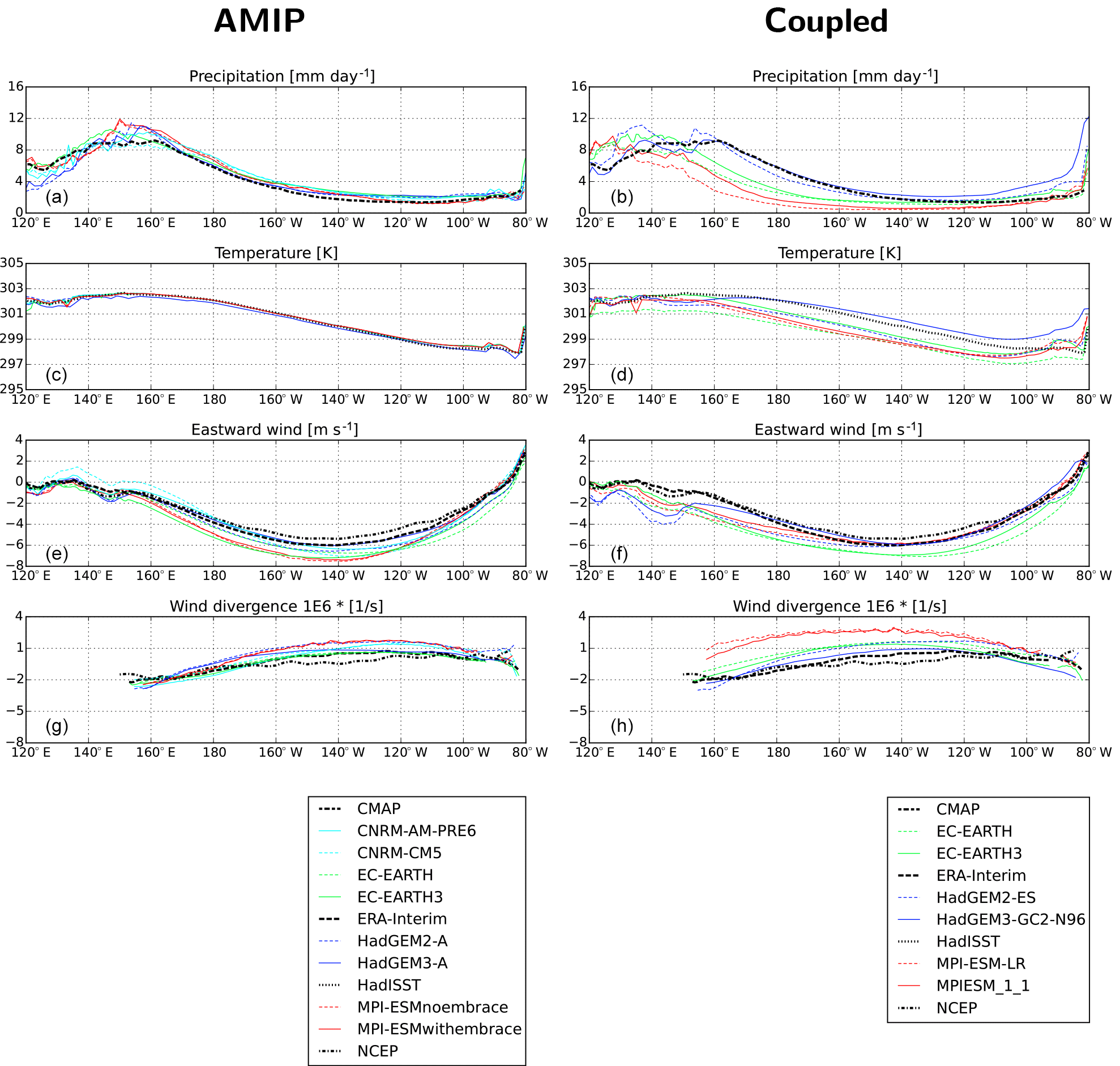
Figure 15Equatorial mean (2.5∘ N to 2.5∘ S) values from top to bottom panels: precipitation, SST, 1000 hPa zonal wind speed, and total 925 hPa wind divergence averaged over the years 1982–2002 (MPI AMIP models 1979–1999). Values are plotted for the equatorial Pacific between 120∘ E and 80∘ W. The left column panels show model results from the AMIP simulations, the right column panels from the coupled (historical) simulations in comparison with observations.
In Fig. 15 we follow the approach from Li and Xie (2014) to analyze the longitudinal structure of the coupled climate simulated in the equatorial Pacific. Figure 15 shows zonal mean precipitation, SST, 1000 hPa zonal wind speed, and 925 hPa wind divergence all averaged between 2.5∘ N and 2.5∘ S from 120∘ E to 80∘ W. As not all ocean data were saved in the EMBRACE simulations, the depth of the ocean 20 ∘C isotherm (as used in Li and Xie, 2014) cannot be plotted and is replaced by 925 hPa wind divergence.
Most AMIP models (left column in Fig. 15) reproduce the zonal structure of precipitation across the Pacific, with minimal values from 80 to 150∘ W and then an increase to a maximum in the western Pacific warm pool region ∼ 145 to 165∘ E. All models, with the possible exception of HadGEM3-A and CNRM-AM-PRE6, simulate too-strong easterly trade winds (too-negative values in Fig. 15), particularly west of 160∘ W. In the AMIP models, this wind bias cannot impact the prescribed SSTs. In the same cross sections for the three coupled simulations (right column), only HadGEM3-GC2 has an accurate zonal structure of SST. All other models have a cold bias of 1 ∘C or more across the central Pacific (between 100∘ W and 170∘ E). Most models also underestimate precipitation in the equatorial band from 150∘ W to 160∘ E and feature a western Pacific rainfall maximum displaced 10–20∘ W of the observed maximum. Only HadGEM3-GC2, and to a lesser extent HadGEM2-ES, capture the correct zonal pattern of precipitation and location of the western Pacific maximum, indicating the important role of SST for the zonal structure of precipitation. Both EC-Earth models show a considerable easterly wind speed bias across most of the Pacific, as does HadGEM2-ES east of 150∘ W. Excess 925 hPa wind divergence is seen in all three coupled models. HadGEM3-GC2 has the most accurate simulation of equatorial zonal wind speeds and wind divergence. This suggests that in the two EC-Earth models and HadGEM2-ES, excessive easterly winds induce too-strong Ekman divergence and ocean upwelling along the equatorial Pacific, leading to the cold SST bias. The two MPI-ESMs have cold SST biases across the Pacific of about 2 ∘C even though the simulated zonal wind speeds are relatively accurate, contrasting significantly with the two AMIP MPI-ESMs in which the largest (positive) easterly wind biases are seen. The cold SST bias in MPI-ESM is accompanied by a positive bias in 925 hPa wind divergence (excessive low-level equatorial divergence), indicating too-strong meridional (poleward directed) wind components near the Equator in this model. The findings suggest excess surface momentum loss from the easterly trade winds, driving both a cold SST bias along the Equator and excessive poleward-directed winds just off the Equator in the MPI coupled models.
Simulated moist convection over the tropical oceans is extremely sensitive to small errors (∼ 0.5 ∘C) in both the absolute value and the spatial gradient of SSTs near the Equator. HadGEM3-GC2 has the most accurate absolute value of tropical SSTs, but suffers from a double-ITCZ problem due its meridional SST gradients across the Equator being incorrect. In contrast, EC-Earth3 has a systematic cold SST bias in both the equatorial Pacific and Atlantic but captures the correct meridional gradient in SST between the two hemispheres. As a result EC-Earth3 does not exhibit a double ITCZ, with a clear precipitation maximum north of the Equator in both basins collocated with SST maxima. Two of the three EMBRACE models (HadGEM3-GC2 and EC-Earth3) show improvement in simulated tropical SSTs compared to their CMIP5 versions. HadGEM3-GC2 in particular has a very accurate zonal structure of SST across the equatorial Pacific, along with associated atmospheric phenomena (precipitation, easterly trade winds). EC-Earth3 also shows some improvement over its CMIP5 version.
3.4 Southern Ocean clouds and radiation
The Southern Ocean plays a key role in the earth's climate, being one of the few extensive regions of the globe where the deep ocean is in regular contact with the surface, allowing for a significant atmosphere–ocean exchange of heat (Kuhlbrodt and Gregory, 2012) and CO2 (Frölicher et al., 2015). Farther south, the formation of Antarctic deep water efficiently transports surface waters into the deep ocean. Both these phenomena are key components of the global ocean overturning circulation (Marshall and Speer, 2012). Trenberth and Fasullo (2010) show that GCMs (CMIP3) have a persistent underestimate in reflected shortwave (SW) radiation at the top of the atmosphere (TOA) over the Southern Ocean, implying that too much SW radiation reaches the ocean surface. Linked to this, many coupled GCMs also show a warm SST bias over extensive parts of the Southern Ocean. This bias increases the vertical stability of the upper ocean and can therefore impact the overturning ocean circulation. Trenberth and Fasullo (2010) and Sallée et al. (2013) suggest that such biases compromise the reliability of climate change projections in the region.
To assess GCM-simulated surface energy budgets over the Southern Ocean, a number of metrics have been implemented into the ESMValTool. In this section we apply some of these metrics to assess the EMBRACE models' ability to capture phenomena controlling the surface radiation budget of the Southern Ocean. We focus on austral summer, when incoming surface radiation is at a maximum and model errors are generally the largest. We analyze total cloud amount, cloud liquid path (LWP) and ice water path (IWP), and surface and TOA solar radiation. Analysis is only performed for the AMIP simulations as the main findings also apply to the coupled models.
Figure 16 shows cross sections from 65 to 30∘ S of simulated zonal mean DJF total cloud cover, LWP and IWP, TOA outgoing (SWUP), and surface downwelling (SWD) shortwave radiation compared to satellite observations. For LWP and IWP, ERA-Interim reanalysis data are also included as a second observationally based estimate (Dee et al., 2011). Observed cloud cover increases from ∼ 60 % at 30∘ S to more than 90 % around 60∘ S. Most models capture this poleward increase, although all except HadGEM3-A exhibit a systematic negative bias (of 5–15 %) across the band ∼ 45 to 65∘ S. HadGEM3-A has the most accurate cloud cover and is a clear improvement over HadGEM2-A. CNRM-AM-PRE6 also shows improvement compared against its CMIP5 version. EC-Earth3 shows a small improvement, while the MPI-ESM shows little change.
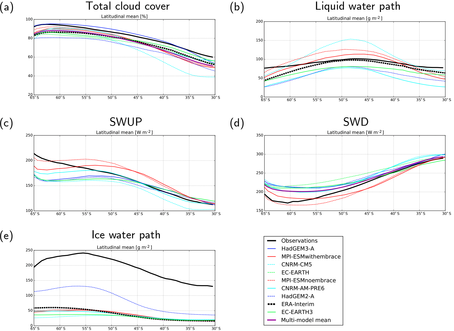
Figure 16Latitude cross section of DJF zonal mean (a) total cloud cover, (b) liquid water path, (c) TOA outgoing shortwave radiation (SWUP), (d) surface downwelling shortwave radiation (SWD), and (e) ice water path. Shown are the CMIP5 and EMBRACE AMIP simulations averaged over the years 1986–2005 (HadGEMs 1986–2004, MPI models 1980–1999) in comparison with satellite observations and the ERA-Interim reanalysis: (a, e) MODIS (2003–2014), (b) UWisc (1988–2007), (c, d) CERES-EBAF (2001–2012).
The impact of clouds on solar radiation can be summarized by cloud optical depth, which is a function of the cloud water content and the effective radius of cloud liquid droplets and ice crystals integrated over cloud depth (Slingo, 1989). Here, vertically integrated LWP values are compared to observed estimates (LWP and IWP are not available from HadGEM3-A or EC-Earth). LWP observations are based on the University of Wisconsin (UWisc; O'Dell et al., 2008) satellite passive microwave dataset, and IWP observations are MODIS collection 6 data (Platnick et al., 2003). Similar to Jiang et al. (2012), the MODIS IWP data representing in-cloud values have been multiplied with the observed ice cloud fraction for comparison with the grid-box averages provided by the models. Due to the large differences across remotely sensed LWP and IWP datasets, values from UWisc and MODIS should be viewed as indicative at best. We include LWP and IWP estimates from ERA-Interim as a second constraint to provide some measure of this uncertainty. Our main motivation is to show the large range in both LWP and IWP across models, which may partly be due to the weak observational constraint.
South of ∼ 40∘ S, LWP differs by a factor of ∼ 2 across models, with IWP showing an even larger inter-model spread (up to a factor of ∼ 3). Such large differences will clearly impact solar radiation fluxes. Before robust guidance on model biases in cloud water biases can be provided for the Southern Ocean, further work is needed to quantify the uncertainty and accuracy of LWP and IWP observations. For now we stress (i) the wide range of LWP and IWP across models and (ii) the lack of a robust observational constraint on these two variables.
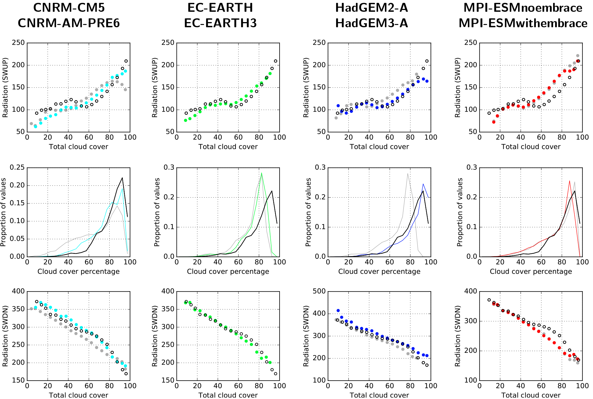
Figure 17Top row panels: scatter plot of monthly mean TOA SWUP versus total cloud cover for the Southern Ocean region 30–65∘ S and season DJF averaged over the years 1986–2005 (MPI models 1980–1999, HadGEMs 1985–2004). Bottom row panels are the same for surface SWDN. Middle row shows fractional occurrence of monthly mean cloud cover over this region. Cloud observations are MODIS-L3 (2003–2014) and SWUP and SWDN are from CERES-EBAF (2001–2014). The EMBRACE-updated AMIP models are plotted in color, the corresponding CMIP5 models are shown in gray, and observations are in black. No radiation data from EC-Earth are available.
Observed SWUP also increases southwards, paralleling the increase in observed cloud cover (Fig. 16a and c). The spread in both SWUP and SWD is decreased going from CMIP5 to the updated models. This is likely primarily a result of the reduced spread (and reduced bias) in cloud cover in the updated models. Nevertheless, a negative bias in SWUP (too little SW reflection) of ∼ 10–40 W m−2 is still seen for all four updated EMBRACE models south of ∼ 55∘ S. This translates into a positive bias in SWD of similar magnitude over the same region. The underestimate in SW reflection for most models is consistent with the (∼ 5–10 %) underestimate of cloud cover south of 55∘ S (only HadGEM3-A does not have a negative bias in cloud cover in this region). The SWUP negative bias is also consistent with an implied underestimate of LWP in EC-Earth3 and CNRM-AM-PRE6 if UWisc data are used as the observational constraint.
To gain more insight into the relationship between cloud cover and reflected SW radiation, Fig. 17 shows scatter plots of monthly mean TOA SWUP and surface SWD each plotted against monthly mean cloud cover for all available DJF months over the 20-year simulation period. Observations are from CERES-EBAF (2001–2014) for SWUP and SWD and MODIS-L3 for cloud cover (2003–2014). The figure is constructed as follows: for each ocean grid point in the band 30 to 65∘ S, monthly cloud cover is binned into 5 % width bins (from 0 and 100 %) and for each cloud cover occurrence the corresponding SWUP and SWD are saved to that bin. This is carried out for all grid points and DJF months, resulting in a mean DJF SWUP and SWD value for each of the 20 cloud cover bins and scatter plots of SWUP and SWD as a function of cloud cover for the region 30 to 65∘ S. The fractional occurrence of cloud cover amounts for each 5 % bin were also recorded and plotted as a frequency distribution (Fig. 17, middle row panels).
The observed cloud cover histogram shows that the bulk of months have cloud cover > 80 %. Most models capture this distribution, with clear improvements in the updated versions of the CNRMs and HadGEMs. EC-Earth3 underestimates the occurrence of cloud cover > 90 %. For the SWUP cloud cover scatter plots, most models underestimate SWUP (and linked to this overestimate SWDN) for cloud cover < 50 %, although the fractional occurrence of cloud cover < 50 % is extremely low (middle row panels in Fig. 17), so this bias may arise from poor sampling and will have minimal impact on the zonal mean SWD and SWUP biases in Fig. 16. All models overestimate SWUP for cloud cover > 60 % (the most frequently occurring cloud amount). These biases range from ∼ 25–30 W m−2 (MPI-ESM) to ∼ 5 W m−2 (HadGEM3-A) and are generally coincident with an underestimate of SWD for the same cloud cover amounts. This finding is not consistent with the zonal mean SWUP and SWD biases seen in Fig. 16, particularly south of ∼ 50∘ S, where all the models underestimate TOA SWUP and overestimate surface SWD ranging from ±10–30 W m−2.
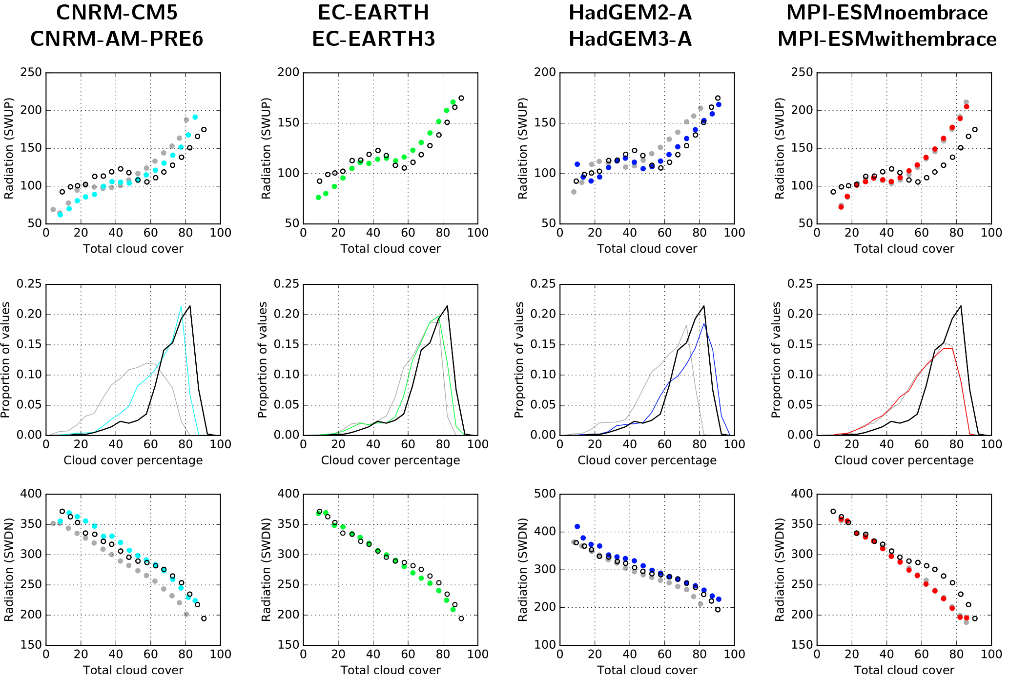
Figure 18As Fig. 17 but for the northern part of the Southern Ocean region (SOC-N, 30–45∘ S).
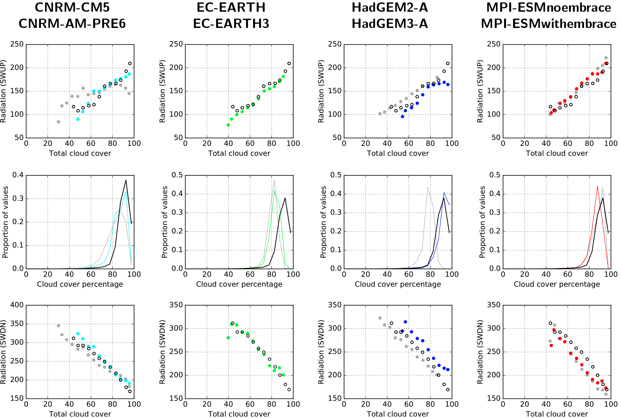
Figure 19As Fig. 17 but for the southern part of the Southern Ocean region (SOC-S, 50–65∘ S).
To understand this inconsistency, Figs. 18 and 19 repeat the radiation–cloud histograms separately for the latitude bands 30–45∘ S (referred to below as SOC-N) and 50–65∘ S (referred to below as SOC-S). For SOC-N the observed cloud histogram is shifted towards lower values, with a peak at 80 % and a tail of occurrences down to 20 %. HadGEM3-A captures this distribution, as does EC-Earth3 to a lesser extent. The other models all show too-frequent cloud cover < 60 % and too-little cloud occurrence > 80 %. The tendency for all models to have a positive bias in TOA SWUP for cloud amounts > 50 % is also seen in this region, although HadGEM3-A is quite accurate in this regard. Figure 16 indicates that the updated EMBRACE models have relatively small zonal mean TOA SWUP and surface SWDN errors in the band 30 to 45∘ S. For the MPI-ESMs and CNRMs, this partly results from error cancellation, with an underestimate of cloud amount balanced by the most frequent cloud amounts (> 50 %) being too reflective. HadGEM3-A has an accurate simulation of zonal mean SWUP and SWD in this latitude band from both accurate cloud amounts and accurate SWUP and SWD cloud cover relationships.
Over the SOC-S region, Fig. 16 shows that all updated models have a negative bias in zonal mean TOA SWUP and a positive bias in surface SWD. The SWUP and SWD cloud cover scatter plots for this region show more mixed results (Fig. 19). This may partly be due to a small sample size, although the main findings we believe are robust. The observed cloud histogram indicates that monthly cloud cover > 90 % dominates at these latitudes. EC-Earth3 and, to a lesser extent, MPI-ESM underestimate the frequency of occurrence of such high cloud amounts, and for these two models this is the leading cause of the negative–positive bias in the SWUP and SWD zonal means. While there is scatter in the observed SWUP and SWD cloud cover relationships over SOC-S, EC-Earth3 and MPI-ESM capture the relationship quite well, suggesting that clouds, when present in these two models in this latitude band, have an accurate representation of SW reflection and transmission. In contrast, CNRM-AM-PRE6 and HadGEM3-A do well in simulating the cloud distribution, but have more mixed success capturing the observed SWUP and SWD cloud relationships. CNRM-AM-PRE6 reproduces this relationship best of these two models. HadGEM3-A reproduces the observed cloud cover histogram very well, but fails to reproduce the SWUP and SWD cloud relationships, with an underestimate in TOA SWUP for cloud > 95 % of ∼ 30–40 W m−2 and a similar error of opposite sign in SWD. This is the leading cause of the zonal mean SWUP and SWD biases in HadGEM3-A.
There is a clear improvement in cloud amounts simulated over the Southern Ocean in the majority of EMBRACE-updated models. This is particularly true for HadGEM3-A compared to HadGEM2-A in which a systematic 10 % underestimate of cloud cover is reduced to close to zero. The CNRM also shows an improvement in cloud amounts across the Southern Ocean. SWUP and SWDN are also surprisingly well captured in most of the updated models, with only the MPI-ESM showing a systematic bias in SWUP (too much reflected SW radiation at TOA) and SWD (too little SWD at the surface) for cloud amounts > 60 %.
Three models show a tendency to compensate for biases (too few clouds balanced by clouds being too reflective), resulting in accurate SWUP and SWD over the 30 to 45∘ S band. Only HadGEM3-A captures both the cloud occurrence distribution SWUP and SWD cloud relationships over this region. Farther south (50 to 65∘ S) most models (apart from EC-Earth3) capture the shift in the most frequent cloud occurrence to > 90 %. In this region models have a greater problem simulating the SWUP and SWD cloud relationships. For example, both HadGEM3-A and CNRM-AM-PRE6 have significant positive biases in surface SWD for cloud amounts of 95–100 %, likely related to an underestimate of cloud optical depth for these cloud types. For further improvement of cloud and radiation processes over the Southern Ocean, improved observational constraints, particularly with respect to in-cloud constituents (e.g., liquid and ice water amounts), are required.
The tropical precipitation in three out of four EMBRACE models analyzed is clearly improved with wet biases in these regions reduced by up to 1–2 mm day−1 compared with the CMIP5 simulations. Precipitation, in particular in tropical regions, remains challenging to model with large biases in the western Pacific and Indian Ocean as well as in the ITCZ and SPCZ. Two of the EMBRACE-updated coupled models exhibit considerable improvements in tropical SSTs, while only one model (EC-Earth3) does not show a double ITCZ in the Pacific.
Biases in the near-surface temperature climatology are still present over many parts of the tropical continents. For example, in most of the analyzed models, a warm bias over Central Africa and northern South America is found. In the coupled simulations, large biases are also still present in the Southern Ocean along the coast of Antarctica. This bias is consistent with the solar radiation biases seen in the four EMBRACE models south of 50∘ S.
The ESMs still have significant problems in accurately simulating all features of the two large-scale atmospheric circulation patterns, the South Asian and West African monsoons. Many of the problems can be traced to difficulties in accurately simulating moist convection over land, interactions between moist convection and (i) convectively forced clouds, impacts on solar radiation, and subsequent surface evaporation and soil water. Initially small biases in moist convection (e.g., in geographical location, intensity, or temporal offsets within the diurnal cycle) can be amplified through these interactions, leading to systematic biases in seasonal mean values. (ii) Convective rainfall and its impact on surface soil water amounts and surface evaporation. Initially small biases can be amplified through feedback processes. For example, rainfall occurring too early in the diurnal cycle (a common bias in many GCMs) will allow a larger fraction of rainfall to be locally evaporated back into the atmosphere instead of percolating into the deeper soil and increasing total soil moisture amounts. A gradual drying out of the surface soil layer will induce upward percolation of soil water and a deepening of the drying signal. The result will be a drying out of soils and a reduced ability to locally sustain moist convection and rainfall, again leading to an amplification of the original bias.
Both feedback loops can be seen as local or regional processes. Once established, these biases can influence the large-scale (surface and mid-tropospheric) thermal gradients driving the monsoon circulation, pushing the simulated monsoon even further from the one observed. The representation of moist convection and its interaction with solar radiation (through convectively forced clouds) and the land surface (through solar radiation and precipitation) are therefore key parameterizations requiring improvement for significant progress in simulating the South Asian and West African monsoons.
Some improvements are seen in the South Asian and West African monsoons from the EMBRACE models compared with their CMIP5 versions. However, significant biases remain, particularly with respect to regional rainfall patterns and the annual cycle of monsoon rainfall. Even more significant biases are seen for intra-seasonal rainfall variability, with little progress from CMIP5 models. In the three coupled model SAM simulations, biases in precipitation and monsoon circulation (given by the 850 hPa wind field) are reduced compared to their CMIP5 counterparts. The primary reason for this is coupled feedbacks that enable the damping of an atmospheric error (e.g., in wind speed or atmospheric moisture content) through the introduction of a compensating bias in surface ocean temperatures (e.g., a cold SST bias). The main model bias regarding West Africa relates to higher-time-frequency precipitation variability on timescales associated with African easterly waves. These systems and the convective complexes embedded within them deliver the majority of rainfall to the West African Sahel. A realistic simulation of AEWs seems an important prerequisite for increasing confidence in future rainfall projections over the Sahel. Most of the EMBRACE models and their CMIP5 versions have severe difficulty in simulating these waves, with little improvement from CMIP5 to the EMBRACE-updated models. The models show quite some spread in their ability to simulate near-surface temperatures over the Sahara, with JJAS mean differences of up to 5 ∘C across models. Given the importance of the Saharan heat low in the overall West African monsoon circulation, more emphasis on simulating the surface energy budget over the Sahara seems necessary. All coupled simulations over West African suffer from excess precipitation at the Guinea coast. This is a direct result of a warm SST bias in all models off the coast of Namibia and Angola. Reduction of this systematic bias, likely through updated ocean physics, resolution, and an improved simulation of marine stratocumulus clouds, will be a necessary step for improving coupled simulations of the West Africa monsoon.
Analysis of AMIP-type simulations performed with EC-Earth at different horizontal resolutions of up to T1279 shows an improvement (i.e., increase) in the variability in precipitation on the synoptic timescale with increasing horizontal resolution up to T511. The seasonal mean rainfall over the WAM and SAM regions, however, does not change significantly with horizontal resolution, suggesting that the reasonably good agreement of modeled and observed mean WAM and SAM rainfall in lower-resolution models may be based on an unrealistic variability and intensity distribution and/or error compensation. The leveling off of the increase in precipitation variability with increasing horizontal model resolution suggests that not all model deficiencies can be solved by going to higher resolutions. Either a resolution higher than T1279 is needed or other non-resolution factors are involved, such as too-simple cloud and precipitation formation parameterizations.
Many models suffer from an excessive cold tongue of water along the Pacific Equator, with this tongue being both too cold and extending too far into the western Pacific. Combined with this cold tongue, coupled models also typically show (i) too-strong easterly trade winds along the Equator, (ii) equatorial rainfall shifted too far west in the western Pacific, (iii) an equatorial thermocline that is too shallow in the eastern Pacific and too deep in the western Pacific, and (iv) a double ITCZ, often with excess rainfall south of the Equator. Comparison of the three EMBRACE coupled models shows a general tendency for improved equatorial SSTs both in the Pacific and Atlantic. HadGEM3-GC2 and EC-Earth3 show improvement in SST bias of as much as 1 ∘C in the zonal and DJF seasonal mean. HadGEM3-GC2, in particular, has a very accurate simulation of tropical SSTs and does not appear to suffer from an excessive equatorial Pacific cold tongue. This is a clear improvement over HadGEM2-ES and is an important reduction in a systematic bias. In combination with the SST improvement, HadGEM3-GC2 also shows a clear improvement in the strength of the easterly trade winds along the Equator. This is likely the primary cause of the reduced SST bias (through reduced Ekman-driven upwelling along the Equator). SSTs in EC-Earth3 are also improved relative to EC-Earth used in CMIP5. Although not as accurate in an absolute sense as HadGEM3-GC2, the meridional structure of SST around the Equator is better in EC-Earth3. This improved spatial structure plays an important role in EC-Earth3 not exhibiting a double ITCZ, with an accurate Northern Hemisphere maximum in precipitation in both the Pacific and Atlantic. Along the equatorial Pacific, EC-Earth3 still suffers from a systematic cold bias (although improved relative to the CMIP5 version of EC-Earth) accompanied by too-strong easterly trade winds.
Most of the EMBRACE-updated models show a clear improvement in monthly cloud cover over the Southern Ocean compared to their CMIP5 predecessors. These improvements feed through into reduced bias (and inter-model spread) in both TOA outgoing solar radiation and surface downwelling solar radiation. A reduction in inter-model spread is also seen for liquid water path, suggesting that the reduced spread translates into reduced model bias, although the observations of LWP over the Southern Ocean suffer from high uncertainties. All four EMBRACE-updated AMIP models have a negative bias in SWUP south of 50∘ S increasing to −20 to −40 W m−2 in the 60 to 65∘ S band. A similar magnitude positive bias in SWD is seen in the same region. While the models show quite some improvement over their CMIP5 counterparts, the SWUP and SWD biases will drive a warm SST bias in the Southern Ocean south of the Antarctic Circumpolar Current (ACC), with negative effects on vertical upwelling and Antarctic deep water formation and sea ice amounts farther south.
The main outstanding cloud–radiation biases appear to be in the southernmost region of the Southern Ocean (e.g., increasing with increasing southerly latitude from 50∘ S). Whether this highlights problems that are specific to certain cloud types (e.g., mid-level clouds in the cold sector of midlatitude weather systems; Bodas-Salcedo et al., 2012), problems in correctly delineating between liquid, solid, and supercooled cloud water (Lawson and Gettelman, 2014), or problems simulating cloud formation in a relative pristine (natural aerosol dominated) region (McCoy et al., 2015) requires further analysis and, in particular, more robust observational constraints.
This analysis has been done with the ESMValTool, which is released under the Apache License version 2.0. The newly added ESMValTool namelist “namelist_lauer18esd.xml” includes the diagnostics that can be used to reproduce the figures in this paper. This version will be available from the ESMValTool webpage at http://www.esmvaltool.org/ and from github (https://github.com/ESMValTool-Core/ESMValTool). Users who apply the software resulting in presentations or papers are kindly asked to cite the ESMValTool documentation paper (Eyring et al., 2016b) along with the software DOI (https://doi.org/10.17874/ac8548f0315) and version number. The climate community is encouraged to contribute to this effort and to join the ESMValTool development team for the contribution of additional diagnostics for ESM evaluation. Data from the CMIP5 models are publically available through the Earth System Grid Federation (ESGF), and the EMBRACE model runs can be made available on request from the host modeling groups.
The supplement related to this article is available online at: https://doi.org/10.5194/esd-9-33-2018-supplement.
The authors declare that they have no conflict of interest.
This work has been performed and funded within the European Commission's
7th Framework Programme under grant agreement number 282672, the “Earth system
Model Bias Reduction and assessing Abrupt Climate change (EMBRACE)” project,
and continued within the European Union's Horizon 2020 research and innovation
programme under grant agreement no. 641816 (CRESCENDO) and the DLR project
“Klimarelevanz von atmosphärischen Spurengasen, Aerosolen und Wolken: Auf
dem Weg zu EarthCARE und MERLIN (KliSAW)”. We acknowledge the World Climate
Research Program (WCRP) Working Group on Coupled Modelling (WGCM), which
is responsible for CMIP, and we thank the climate modeling groups for producing
and making available their model output. For CMIP5 the US Department of Energy's
Program for Climate Model Diagnosis and Intercomparison provides coordinating
support and led the development of software infrastructure in partnership with the
Global Organization for Earth System Science Portals. Romain Roehrig acknowledges
the work of the CNRM climate model development team, which contributed to the
development of the CNRM-AM-PRE6 prototype version used in the present study.
He also acknowledges support from the French national program LEFE/INSU under
the DEPHY2 project.
The article processing charges for this open-access
publication
were covered by a Research
Centre of the Helmholtz Association.
Edited by: Gerrit Lohmann
Reviewed by: two anonymous referees
Adler, R. F., Huffman, G. J., Chang, A., Ferraro, R., Xie, P. P., Janowiak, J., Rudolf, B., Schneider, U., Curtis, S., Bolvin, D., Gruber, A., Susskind, J., Arkin, P., and Nelkin, E.: The version-2 global precipitation climatology project (GPCP) monthly precipitation analysis (1979–present), J. Hydrometeorol., 4, 1147–1167, https://doi.org/10.1175/1525-7541(2003)004<1147:Tvgpcp>2.0.Co;2, 2003.
Bechtold, P., Semane, N., Lopez, P., Chaboureau, J. P., Beljaars, A., and Bormann, N.: Representing Equilibrium and Nonequilibrium Convection in Large-Scale Models, J. Atmos. Sci., 71, 734–753, https://doi.org/10.1175/Jas-D-13-0163.1, 2014.
Bellenger, H., Guilyardi, E., Leloup, J., Lengaigne, M., and Vialard, J.: ENSO representation in climate models: from CMIP3 to CMIP5, Clim. Dynam., 42, 1999–2018, https://doi.org/10.1007/s00382-013-1783-z, 2014.
Biasutti, M.: Forced Sahel rainfall trends in the CMIP5 archive, J. Geophys. Res.-Atmos., 118, 1613–1623, https://doi.org/10.1002/jgrd.50206, 2013.
Bjerknes, J.: Atmospheric teleconnections from the equatorial Pacific, Mon. Weather Rev., 97, 163–172, https://doi.org/10.1175/1520-0493(1969)097<0163:atftep>2.3.co;2, 1969.
Bodas-Salcedo, A., Williams, K. D., Field, P. R., and Lock, A. P.: The Surface Downwelling Solar Radiation Surplus over the Southern Ocean in the Met Office Model: The Role of Midlatitude Cyclone Clouds, J. Climate, 25, 7467–7486, https://doi.org/10.1175/Jcli-D-11-00702.1, 2012.
Caniaux, G., Giordani, H., Redelsperger, J. L., Guichard, F., Key, E., and Wade, M.: Coupling between the Atlantic cold tongue and the West African monsoon in boreal spring and summer, J. Geophys. Res.-Oceans, 116, C04003, https://doi.org/10.1029/2010jc006570, 2011.
Chang, C.-P., Wang, Z., and Hendon, H.: The Asian winter monsoon, in: The Asian Monsoon, edited by: Wang, B., Springer-Verlag, Berlin, Heidelberg, 89–126, 2006.
Collins, M., An, S. I., Cai, W. J., Ganachaud, A., Guilyardi, E., Jin, F. F., Jochum, M., Lengaigne, M., Power, S., Timmermann, A., Vecchi, G., and Wittenberg, A.: The impact of global warming on the tropical Pacific ocean and El Nino, Nat. Geosci., 3, 391–397, https://doi.org/10.1038/Ngeo868, 2010.
Collins, W. J., Bellouin, N., Doutriaux-Boucher, M., Gedney, N., Halloran, P., Hinton, T., Hughes, J., Jones, C. D., Joshi, M., Liddicoat, S., Martin, G., O'Connor, F., Rae, J., Senior, C., Sitch, S., Totterdell, I., Wiltshire, A., and Woodward, S.: Development and evaluation of an Earth-System model-HadGEM2, Geosci. Model Dev., 4, 1051–1075, https://doi.org/10.5194/gmd-4-1051-2011, 2011.
Cuxart, J., Bougeault, P., and Redelsperger, J. L.: A turbulence scheme allowing for mesoscale and large-eddy simulations, Q. J. Roy. Meteorol. Soc., 126, 1–30, https://doi.org/10.1002/qj.49712656202, 2000.
Dawson, A. and Palmer, T. N.: Simulating weather regimes: impact of model resolution and stochastic parameterization, Clim. Dynam., 44, 2177–2193, https://doi.org/10.1007/s00382-014-2238-x, 2015.
Dee, D. P., Uppala, S. M., Simmons, A. J., Berrisford, P., Poli, P., Kobayashi, S., Andrae, U., Balmaseda, M. A., Balsamo, G., Bauer, P., Bechtold, P., Beljaars, A. C. M., van de Berg, L., Bidlot, J., Bormann, N., Delsol, C., Dragani, R., Fuentes, M., Geer, A. J., Haimberger, L., Healy, S. B., Hersbach, H., Holm, E. V., Isaksen, L., Kallberg, P., Kohler, M., Matricardi, M., McNally, A. P., Monge-Sanz, B. M., Morcrette, J. J., Park, B. K., Peubey, C., de Rosnay, P., Tavolato, C., Thepaut, J. N., and Vitart, F.: The ERA-Interim reanalysis: configuration and performance of the data assimilation system, Q. J. Roy. Meteorol. Soc., 137, 553–597, https://doi.org/10.1002/qj.828, 2011.
Demory, M. E., Vidale, P. L., Roberts, M. J., Berrisford, P., Strachan, J., Schiemann, R., and Mizielinski, M. S.: The role of horizontal resolution in simulating drivers of the global hydrological cycle, Clim. Dynam., 42, 2201–2225, https://doi.org/10.1007/s00382-013-1924-4, 2014.
de Szoeke, S. P., Fairall, C. W., Wolfe, D. E., Bariteau, L., and Zuidema, P.: Surface Flux Observations on the Southeastern Tropical Pacific Ocean and Attribution of SST Errors in Coupled Ocean-Atmosphere Models, J. Climate, 23, 4152–4174, https://doi.org/10.1175/2010jcli3411.1, 2010.
England, M. H., McGregor, S., Spence, P., Meehl, G. A., Timmermann, A., Cai, W. J., Sen Gupta, A., McPhaden, M. J., Purich, A., and Santoso, A.: Recent intensification of wind-driven circulation in the Pacific and the ongoing warming hiatus, Nat. Clim. Change, 4, 222–227, https://doi.org/10.1038/Nclimate2106, 2014.
Eyring, V., Bony, S., Meehl, G. A., Senior, C. A., Stevens, B., Stouffer, R. J., and Taylor, K. E.: Overview of the Coupled Model Intercomparison Project Phase 6 (CMIP6) experimental design and organization, Geosci. Model Dev., 9, 1937–1958, https://doi.org/10.5194/gmd-9-1937-2016, 2016a.
Eyring, V., Righi, M., Lauer, A., Evaldsson, M., Wenzel, S., Jones, C., Anav, A., Andrews, O., Cionni, I., Davin, E. L., Deser, C., Ehbrecht, C., Friedlingstein, P., Gleckler, P., Gottschaldt, K. D., Hagemann, S., Juckes, M., Kindermann, S., Krasting, J., Kunert, D., Levine, R., Loew, A., Makela, J., Martin, G., Mason, E., Phillips, A. S., Read, S., Rio, C., Roehrig, R., Senftleben, D., Sterl, A., van Ulft, L. H., Walton, J., Wang, S. Y., and Williams, K. D.: ESMValTool (v1.0) – a community diagnostic and performance metrics tool for routine evaluation of Earth system models in CMIP, Geosci. Model Dev., 9, 1747–1802, https://doi.org/10.5194/gmd-9-1747-2016, 2016b.
Fink, A. H. and Reiner, A.: Spatiotemporal variability of the relation between African Easterly Waves and West African Squall Lines in 1998 and 1999, J. Geophys. Res.-Atmos., 108, 4332, https://doi.org/10.1029/2002jd002816, 2003.
Flato, G., Marotzke, J., Abiodun, B., Braconnot, P., Chou, S. C., Collins, W., Cox, P., Driouech, F., Emori, S., Eyring, V., Forest, C., Gleckler, P., Guilyardi, E., Jakob, C., Kattsov, V., Reason, C., and Rummukainen, M.: Evaluation of Climate Models, in: Climate Change 2013: The Physical Science Basis, Contribution of Working Group I to the Fifth Assessment Report of the Intergovernmental Panel on Climate Change, edited by: Stocker, T. F., Qin, D., Plattner, G.-K., Tignor, M., Allen, S. K., Boschung, J., Nauels, A., Xia, Y., Bex, V., and Midgley, P. M., Cambridge University Press, Cambridge, UK and New York, NY, USA, 741–866, 2013.
Forbes, R. M., Tompkins, A., and Untch, A.: A new prognostic bulk microphysics scheme for the IFS, ECMWF TM 9441, http://www.ecmwf.int/sites/default/files/elibrary/2011/9441-new-prognostic-bulk-microphysics-scheme-ifs.pdf (last access: January 2017), 2011.
Frierson, D. M. W. and Hwang, Y. T.: Extratropical Influence on ITCZ Shifts in Slab Ocean Simulations of Global Warming, J. Climate, 25, 720–733, https://doi.org/10.1175/Jcli-D-11-00116.1, 2012.
Frierson, D. M. W., Hwang, Y. T., Fuckar, N. S., Seager, R., Kang, S. M., Donohoe, A., Maroon, E. A., Liu, X. J., and Battisti, D. S.: Contribution of ocean overturning circulation to tropical rainfall peak in the Northern Hemisphere, Nat. Geosci., 6, 940–944, https://doi.org/10.1038/Ngeo1987, 2013.
Frölicher, T. L., Sarmiento, J. L., Paynter, D. J., Dunne, J. P., Krasting, J. P., and Winton, M.: Dominance of the Southern Ocean in Anthropogenic Carbon and Heat Uptake in CMIP5 Models, J. Climate, 28, 862–886, https://doi.org/10.1175/Jcli-D-14-00117.1, 2015.
Goll, D. S., Brovkin, V., Liski, J., Raddatz, T., Thum, T., and Todd-Brown, K. E. O.: Strong dependence of CO2 emissions from anthropogenic land cover change on initial land cover and soil carbon parametrization, Global Biogeochem. Cy., 29, 1511–1523, https://doi.org/10.1002/2014gb004988, 2015.
Goswami, B. N., Krishnamurthy, V., and Annamalai, H.: A broad-scale circulation index for the interannual variability of the Indian summer monsoon, Q. J. Roy. Meteorol. Soc., 125, 611–633, https://doi.org/10.1256/smsqj.55411, 1999.
Graham, F. S., Brown, J. N., Langlais, C., Marsland, S. J., Wittenberg, A. T., and Holbrook, N. J.: Effectiveness of the Bjerknes stability index in representing ocean dynamics, Clim. Dynam., 43, 2399–2414, https://doi.org/10.1007/s00382-014-2062-3, 2014.
Graham, F. S., Brown, J. N., Wittenberg, A. T., and Holbrook, N. J.: Reassessing Conceptual Models of ENSO, J. Climate, 28, 9121–9142, https://doi.org/10.1175/Jcli-D-14-00812.1, 2015.
Guérémy, J. F.: A continuous buoyancy based convection scheme: one- and three-dimensional validation, Tellus A, 63, 687–706, https://doi.org/10.1111/j.1600-0870.2011.00521.x, 2011.
Guilyardi, E.: El Niño-mean state-seasonal cycle interactions in a multi-model ensemble, Clim. Dynam., 26, 329–348, https://doi.org/10.1007/s00382-005-0084-6, 2006.
Hagemann, S. and Stacke, T.: Impact of the soil hydrology scheme on simulated soil moisture memory, Clim. Dynam., 44, 1731–1750, https://doi.org/10.1007/s00382-014-2221-6, 2015.
Harris, I., Jones, P. D., Osborn, T. J., and Lister, D. H.: Updated high-resolution grids of monthly climatic observations – the CRU TS3.10 Dataset, Int. J. Climatol., 34, 623–642, https://doi.org/10.1002/joc.3711, 2014.
Hazeleger, W., Guemas, V., Wouters, B., Corti, S., Andreu-Burillo, I., Doblas-Reyes, F. J., Wyser, K., and Caian, M.: Multiyear climate predictions using two initialization strategies, Geophys. Res. Lett., 40, 1794–1798, https://doi.org/10.1002/grl.50355, 2013.
Heidinger, A. K., Foster, M. J., Walther, A., and Zhao, X. P.: The Pathfinder Atmospheres-Extended AVHRR Climate Dataset, B. Am. Meteorol. Soc., 95, 909–922, https://doi.org/10.1175/Bams-D-12-00246.1, 2014.
Held, I. M., Delworth, T. L., Lu, J., Findell, K. L., and Knutson, T. R.: Simulation of Sahel drought in the 20th and 21st centuries, P. Natl. Acad. Sci. USA, 102, 17891–17896, https://doi.org/10.1073/pnas.0509057102, 2005.
Huang, B. H., Hu, Z. Z., and Jha, B.: Evolution of model systematic errors in the Tropical Atlantic Basin from coupled climate hindcasts, Clim. Dynam., 28, 661–682, https://doi.org/10.1007/s00382-006-0223-8, 2007.
Huffman, G. J. and Bolvin, D. T.: GPCP Version 2.2 SG Combined Precipitation Data Set Documentation, available at: ftp://precip.gsfc.nasa.gov/pub/gpcp-v2.2/doc/V2.2_doc.pdf (last access: January 2016), 2012.
Huffman, G. J., Adler, R. F., Morrissey, M. M., Bolvin, D. T., Curtis, S., Joyce, R., McGavock, B., and Susskind, J.: Global precipitation at one-degree daily resolution from multisatellite observations, J. Hydrometeorol., 2, 36–50, https://doi.org/10.1175/1525-7541(2001)002<0036:Gpaodd>2.0.Co;2, 2001.
Huffman, G. J., Adler, R. F., Bolvin, D. T., Gu, G. J., Nelkin, E. J., Bowman, K. P., Hong, Y., Stocker, E. F., and Wolff, D. B.: The TRMM multisatellite precipitation analysis (TMPA): Quasi-global, multiyear, combined-sensor precipitation estimates at fine scales, J. Hydrometeorol., 8, 38–55, https://doi.org/10.1175/Jhm560.1, 2007.
Hunt, K. M. R., Turner, A. G., and Parker, D. E.: The spatiotemporal structure of precipitation in Indian monsoon depressions, Q. J. Roy. Meteorol. Soc., 142, 3195–3210, https://doi.org/10.1002/qj.2901, 2016.
Jiang, J. H., Su, H., Zhai, C. X., Perun, V. S., Del Genio, A., Nazarenko, L. S., Donner, L. J., Horowitz, L., Seman, C., Cole, J., Gettelman, A., Ringer, M. A., Rotstayn, L., Jeffrey, S., Wu, T. W., Brient, F., Dufresne, J. L., Kawai, H., Koshiro, T., Watanabe, M., LEcuyer, T. S., Volodin, E. M., Iversen, T., Drange, H., Mesquita, M. D. S., Read, W. G., Waters, J. W., Tian, B. J., Teixeira, J., and Stephens, G. L.: Evaluation of cloud and water vapor simulations in CMIP5 climate models using NASA “A-Train” satellite observations, J. Geophys. Res.-Atmos., 117, D14105, https://doi.org/10.1029/2011jd017237, 2012.
Jung, T., Balsamo, G., Bechtold, P., Beljaars, A. C. M., Köhler, M., Miller, M. J., Morcrette, J.-J., Orr, A., Rodwell, M., and Tompkins, A. M.: The ECMWF model climate: Recent progress through improved physical parametrizations, ECMWF TM 10317, http://www.ecmwf.int/sites/default/files/elibrary/2010/10317 (last access: January 2017), 2010.
Jung, T., Miller, M. J., Palmer, T. N., Towers, P., Wedi, N., Achuthavarier, D., Adams, J. M., Altshuler, E. L., Cash, B. A., Kinter, J. L., Marx, L., Stan, C., and Hodges, K. I.: High-Resolution Global Climate Simulations with the ECMWF Model in Project Athena: Experimental Design, Model Climate, and Seasonal Forecast Skill, J. Climate, 25, 3155–3172, https://doi.org/10.1175/Jcli-D-11-00265.1, 2012.
Jungclaus, J. H., Fischer, N., Haak, H., Lohmann, K., Marotzke, J., Matei, D., Mikolajewicz, U., Notz, D., and von Storch, J. S.: Characteristics of the ocean simulations in the Max Planck Institute Ocean Model (MPIOM) the ocean component of the MPI-Earth system model, J. Adv. Model Earth Syst., 5, 422–446, https://doi.org/10.1002/jame.20023, 2013.
Kalnay, E., Kanamitsu, M., Kistler, R., Collins, W., Deaven, D., Gandin, L., Iredell, M., Saha, S., White, G., Woollen, J., Zhu, Y., Chelliah, M., Ebisuzaki, W., Higgins, W., Janowiak, J., Mo, K. C., Ropelewski, C., Wang, J., Leetmaa, A., Reynolds, R., Jenne, R., and Joseph, D.: The NCEP/NCAR 40-year reanalysis project, B. Am. Meteorol. Soc., 77, 437–471, https://doi.org/10.1175/1520-0477(1996)077<0437:Tnyrp>2.0.Co;2, 1996.
Kang, I. S., Jin, K., Wang, B., Lau, K. M., Shukla, J., Krishnamurthy, V., Schubert, S. D., Wailser, D. E., Stern, W. F., Kitoh, A., Meehl, G. A., Kanamitsu, M., Galin, V. Y., Satyan, V., Park, C. K., and Liu, Y.: Intercomparison of the climatological variations of Asian summer monsoon precipitation simulated by 10 GCMs, Clim. Dynam., 19, 383–395, https://doi.org/10.1007/s00382-002-0245-9, 2002.
Kang, S. M., Frierson, D. M. W., and Held, I. M.: The Tropical Response to Extratropical Thermal Forcing in an Idealized GCM: The Importance of Radiative Feedbacks and Convective Parameterization, J. Atmos. Sci., 66, 2812–2827, https://doi.org/10.1175/2009jas2924.1, 2009.
Kiladis, G. N., Thorncroft, C. D., and Hall, N. M. J.: Three-dimensional structure and dynamics of African easterly waves. Part I: Observations, J. Atmos. Sci., 63, 2212–2230, https://doi.org/10.1175/Jas3741.1, 2006.
Kuhlbrodt, T. and Gregory, J. M.: Ocean heat uptake and its consequences for the magnitude of sea level rise and climate change, Geophys. Res. Lett., 39, L18608, https://doi.org/10.1029/2012gl052952, 2012.
Lauer, A. and Hamilton, K.: Simulating Clouds with Global Climate Models: A Comparison of CMIP5 Results with CMIP3 and Satellite Data, J. Climate, 26, 3823–3845, https://doi.org/10.1175/Jcli-D-12-00451.1, 2013.
Lavaysse, C., Flamant, C., Janicot, S., Parker, D. J., Lafore, J. P., Sultan, B., and Pelon, J.: Seasonal evolution of the West African heat low: a climatological perspective, Clim. Dynam., 33, 313–330, https://doi.org/10.1007/s00382-009-0553-4, 2009.
Lawson, R. P. and Gettelman, A.: Impact of Antarctic mixed-phase clouds on climate, P. Natl. Acad. Sci. USA, 111, 18156–18161, https://doi.org/10.1073/pnas.1418197111, 2014.
Levine, R. C. and Turner, A. G.: Dependence of Indian monsoon rainfall on moisture fluxes across the Arabian Sea and the impact of coupled model sea surface temperature biases, Clim. Dynam., 38, 2167–2190, https://doi.org/10.1007/s00382-011-1096-z, 2012.
Levine, R. C., Turner, A. G., Marathayil, D., and Martin, G. M.: The role of northern Arabian Sea surface temperature biases in CMIP5 model simulations and future projections of Indian summer monsoon rainfall, Clim. Dynam., 41, 155–172, https://doi.org/10.1007/s00382-012-1656-x, 2013.
Li, G. and Xie, S. P.: Tropical Biases in CMIP5 Multimodel Ensemble: The Excessive Equatorial Pacific Cold Tongue and Double ITCZ Problems, J. Climate, 27, 1765–1780, https://doi.org/10.1175/Jcli-D-13-00337.1, 2014.
Lin, J. L.: The double-ITCZ problem in IPCC AR4 coupled GCMs: Ocean–atmosphere feedback analysis, J. Climate, 20, 4497–4525, https://doi.org/10.1175/Jcli4272.1, 2007.
Loeb, N. G., Wielicki, B. A., Doelling, D. R., Smith, G. L., Keyes, D. F., Kato, S., Manalo-Smith, N., and Wong, T.: Toward Optimal Closure of the Earth's Top-of-Atmosphere Radiation Budget, J. Climate, 22, 748–766, https://doi.org/10.1175/2008jcli2637.1, 2009.
Loeb, N. G., Lyman, J. M., Johnson, G. C., Allan, R. P., Doelling, D. R., Wong, T., Soden, B. J., and Stephens, G. L.: Observed changes in top-of-the-atmosphere radiation and upper-ocean heating consistent within uncertainty, Nat. Geosci., 5, 110–113, https://doi.org/10.1038/Ngeo1375, 2012.
Lopez, P.: Implementation and validation of a new prognostic large-scale cloud and precipitation scheme for climate and data-assimilation purposes, Q. J. Roy. Meteorol. Soc., 128, 229–257, https://doi.org/10.1256/00359000260498879, 2002.
Marshall, J. and Speer, K.: Closure of the meridional overturning circulation through Southern Ocean upwelling, Nat. Geosci., 5, 171–180, https://doi.org/10.1038/Ngeo1391, 2012.
Marshall, J., Donohoe, A., Ferreira, D., and McGee, D.: The ocean's role in setting the mean position of the Inter-Tropical Convergence Zone, Clim. Dynam., 42, 1967–1979, https://doi.org/10.1007/s00382-013-1767-z, 2014.
Martin, G. M., Bellouin, N., Collins, W. J., Culverwell, I. D., Halloran, P. R., Hardiman, S. C., Hinton, T. J., Jones, C. D., McDonald, R. E., McLaren, A. J., O'Connor, F. M., Roberts, M. J., Rodriguez, J. M., Woodward, S., Best, M. J., Brooks, M. E., Brown, A. R., Butchart, N., Dearden, C., Derbyshire, S. H., Dharssi, I., Doutriaux-Boucher, M., Edwards, J. M., Falloon, P. D., Gedney, N., Gray, L. J., Hewitt, H. T., Hobson, M., Huddleston, M. R., Hughes, J., Ineson, S., Ingram, W. J., James, P. M., Johns, T. C., Johnson, C. E., Jones, A., Jones, C. P., Joshi, M. M., Keen, A. B., Liddicoat, S., Lock, A. P., Maidens, A. V., Manners, J. C., Milton, S. F., Rae, J. G. L., Ridley, J. K., Sellar, A., Senior, C. A., Totterdell, I. J., Verhoef, A., Vidale, P. L., Wiltshire, A., and Team, H. D.: The HadGEM2 family of Met Office Unified Model climate configurations, Geosci. Model Dev., 4, 723–757, https://doi.org/10.5194/gmd-4-723-2011, 2011.
Martin, G. M., Peyrille, P., Roehrig, R., Rio, C., Caian, M., Bellon, G., Codron, F., Lafore, J. P., Poan, D. E., and Idelkadi, A.: Understanding the West African Monsoon from the analysis of diabatic heating distributions as simulated by climate models, J. Adv. Model Earth Syst., 9, 239–270, https://doi.org/10.1002/2016ms000697, 2017.
Mathon, V., Laurent, H., and Lebel, T.: Mesoscale convective system rainfall in the Sahel, J. Appl. Meteorol., 41, 1081–1092, https://doi.org/10.1175/1520-0450(2002)041<1081:Mcsrit>2.0.Co;2, 2002.
McCoy, D. T., Burrows, S. M., Wood, R., Grosvenor, D. P., Elliott, S. M., Ma, P.-L., Rasch, P. J., and Hartmann, D. L.: Natural aerosols explain seasonal and spatial patterns of Southern Ocean cloud albedo, Sci. Adv., 1, e1500157, https://doi.org/10.1126/sciadv.1500157, 2015.
Meehl, G. A., Arblaster, J. M., Fasullo, J. T., Hu, A. X., and Trenberth, K. E.: Model-based evidence of deep-ocean heat uptake during surface-temperature hiatus periods, Nat. Clim. Change, 1, 360–364, https://doi.org/10.1038/Nclimate1229, 2011.
Megann, A., Storkey, D., Aksenov, Y., Alderson, S., Calvert, D., Graham, T., Hyder, P., Siddorn, J., and Sinha, B.: GO5.0: the joint NERC-Met Office NEMO global ocean model for use in coupled and forced applications, Geosci. Model Dev., 7, 1069–1092, https://doi.org/10.5194/gmd-7-1069-2014, 2014.
Menon, A., Levermann, A., and Schewe, J.: Enhanced future variability during India's rainy season, Geophys. Res. Lett., 40, 3242–3247, https://doi.org/10.1002/grl.50583, 2013.
Michou, M., Nabat, P., and Saint-Martin, D.: Development and basic evaluation of a prognostic aerosol scheme (v1) in the CNRM Climate Model CNRM-CM6, Geosci. Model Dev., 8, 501–531, https://doi.org/10.5194/gmd-8-501-2015, 2015.
Neelin, J. D. and Dijkstra, H. A.: Ocean-Atmosphere Interaction and the Tropical Climatology. 1. The Dangers of Flux Correction, J. Climate, 8, 1325–1342, https://doi.org/10.1175/1520-0442(1995)008<1325:Oaiatt>2.0.Co;2, 1995.
Nicholson, S. E. and Grist, J. P.: The seasonal evolution of the atmospheric circulation over West Africa and equatorial Africa, J. Climate, 16, 1013–1030, https://doi.org/10.1175/1520-0442(2003)016<1013:Tseota>2.0.Co;2, 2003.
Nicholson, S. E., Some, B., and Kone, B.: An analysis of recent rainfall conditions in West Africa, including the rainy seasons of the 1997 El Nino and the 1998 La Nina years, J. Climate, 13, 2628–2640, https://doi.org/10.1175/1520-0442(2000)013<2628:Aaorrc>2.0.Co;2, 2000.
O'Dell, C. W., Wentz, F. J., and Bennartz, R.: Cloud liquid water path from satellite-based passive microwave observations: A new climatology over the global oceans, J. Climate, 21, 1721–1739, https://doi.org/10.1175/2007jcli1958.1, 2008.
Oueslati, B. and Bellon, G.: The double ITCZ bias in CMIP5 models: interaction between SST, large-scale circulation and precipitation, Clim. Dynam., 44, 585–607, https://doi.org/10.1007/s00382-015-2468-6, 2015.
Penland, C. and Sardeshmukh, P. D.: The Optimal-Growth of Tropical Sea-Surface Temperature Anomalies, J. Climate, 8, 1999–2024, https://doi.org/10.1175/1520-0442(1995)008<1999:Togots>2.0.Co;2, 1995.
Piriou, J. M., Redelsperger, J. L., Geleyn, J. F., Lafore, J. P., and Guichard, F.: An approach for convective parameterization with memory: Separating microphysics and transport in grid-scale equations, J. Atmos. Sci., 64, 4127–4139, https://doi.org/10.1175/2007jas2144.1, 2007.
Platnick, S., King, M. D., Ackerman, S. A., Menzel, W. P., Baum, B. A., Riedi, J. C., and Frey, R. A.: The MODIS cloud products: Algorithms and examples from Terra, IEEE T. Geosci. Remote, 41, 459–473, https://doi.org/10.1109/Tgrs.2002.808301, 2003.
Platnick, S., et al.: MODIS Atmosphere L3 Monthly Product MYD08_M3, NASA MODIS Adaptive Processing System, Goddard Space Flight Center, USA, https://doi.org/10.5067/MODIS/MYD08_M3.006, 2015.
Poan, D. E., Roehrig, R., Couvreux, F., and Lafore, J. P.: West African Monsoon Intraseasonal Variability: A Precipitable Water Perspective, J. Atmos. Sci., 70, 1035–1052, https://doi.org/10.1175/Jas-D-12-087.1, 2013.
Poan, D. E., Lafore, J. P., Roehrig, R., and Couvreux, F.: Internal processes within the African Easterly Wave system, Q. J. Roy. Meteorol. Soc., 141, 1121–1136, https://doi.org/10.1002/qj.2420, 2015.
Rae, J. G. L., Hewitt, H. T., Keen, A. B., Ridley, J. K., West, A. E., Harris, C. M., Hunke, E. C., and Walters, D. N.: Development of the Global Sea Ice 6.0 CICE configuration for the Met Office Global Coupled model, Geosci. Model Dev., 8, 2221–2230, https://doi.org/10.5194/gmd-8-2221-2015, 2015.
Randall, D. A., Wood, R. A., Bony, S., Colman, R., Fichefet, T., Fyfe, J., Kattsov, V., Pitman, A., Shukla, J., Srinivasan, J., Stouffer, R. J., Sumi, A., and Taylor, K. E.: Climate Models and Their Evaluation, Climate Change 2007: The Physical Science Basis, in: Contribution of Working Group I to the Fourth Assessment Report of the Intergovernmental Panel on Climate Change, edited by: Solomon, S., Qin, D., Manning, M., Chen, Z., Marquis, M., Averyt, K. B., Tignor, M., and Miller, H. L., Cambridge University Press, Cambridge, UK and New York, NY, USA, 2007.
Rayner, N. A., Parker, D. E., Horton, E. B., Folland, C. K., Alexander, L. V., Rowell, D. P., Kent, E. C., and Kaplan, A.: Global analyses of sea surface temperature, sea ice, and night marine air temperature since the late nineteenth century, J. Geophys. Res.-Atmos., 108,4407, https://doi.org/10.1029/2002jd002670, 2003.
Reynolds, R. W., Smith, T. M., Liu, C., Chelton, D. B., Casey, K. S., and Schlax, M. G.: Daily high-resolution-blended analyses for sea surface temperature, J. Climate, 20, 5473–5496, https://doi.org/10.1175/2007jcli1824.1, 2007.
Richter, I. and Xie, S. P.: On the origin of equatorial Atlantic biases in coupled general circulation models, Clim. Dynam., 31, 587–598, https://doi.org/10.1007/s00382-008-0364-z, 2008.
Roberts, M. J., Vidale, P. L., Mizielinski, M. S., Demory, M. E., Schiemann, R., Strachan, J., Hodges, K., Bell, R., and Camp, J.: Tropical Cyclones in the UPSCALE Ensemble of High-Resolution Global Climate Models, J. Climate, 28, 574–596, https://doi.org/10.1175/Jcli-D-14-00131.1, 2015.
Roehrig, R., Bouniol, D., Guichard, F., Hourdin, F., and Redelsperger, J. L.: The Present and Future of the West African Monsoon: A Process-Oriented Assessment of CMIP5 Simulations along the AMMA Transect, J. Climate, 26, 6471–6505, https://doi.org/10.1175/Jcli-D-12-00505.1, 2013.
Ruti, P. M. and Dell'Aquila, A.: The twentieth century African easterly waves in reanalysis systems and IPCC simulations, from intra-seasonal to inter-annual variability, Clim. Dynam., 35, 1099–1117, https://doi.org/10.1007/s00382-010-0894-z, 2010.
Saeed, F., Hagemann, S., and Jacob, D.: Impact of irrigation on the South Asian summer monsoon, Geophys. Res. Lett., 36, L20711, https://doi.org/10.1029/2009gl040625, 2009.
Sallée, J. B., Shuckburgh, E., Bruneau, N., Meijers, A. J. S., Bracegirdle, T. J., and Wang, Z.: Assessment of Southern Ocean mixed-layer depths in CMIP5 models: Historical bias and forcing response, J. Geophys. Res.-Oceans, 118, 1845–1862, https://doi.org/10.1002/jgrc.20157, 2013.
Scaife, A. A., Butchart, N., Warner, C. D., and Swinbank, R.: Impact of a spectral gravity wave parameterization on the stratosphere in the met office unified model, J. Atmos. Sci., 59, 1473–1489, https://doi.org/10.1175/1520-0469(2002)059<1473:Ioasgw>2.0.Co;2, 2002.
Shu, Q., Song, Z., and Qiao, F.: Assessment of sea ice simulations in the CMIP5 models, The Cryosphere, 9, 399–409, https://doi.org/10.5194/tc-9-399-2015, 2015.
Slingo, A.: A GCM Parameterization for the Shortwave Radiative Properties of Water Clouds, J. Atmos. Sci., 46, 1419–1427, https://doi.org/10.1175/1520-0469(1989)046<1419:Agpfts>2.0.Co;2, 1989.
Stevens, B., Giorgetta, M., Esch, M., Mauritsen, T., Crueger, T., Rast, S., Salzmann, M., Schmidt, H., Bader, J., Block, K., Brokopf, R., Fast, I., Kinne, S., Kornblueh, L., Lohmann, U., Pincus, R., Reichler, T., and Roeckner, E.: Atmospheric component of the MPI-M Earth System Model: ECHAM6, J. Adv. Model Earth Syst., 5, 146–172, https://doi.org/10.1002/jame.20015, 2013.
Sultan, B. and Janicot, S.: The West African monsoon dynamics. Part II: The “preonset” and “onset” of the summer monsoon, J. Climate, 16, 3407–3427, https://doi.org/10.1175/1520-0442(2003)016<3407:Twamdp>2.0.Co;2, 2003.
Taylor, K. E., Stouffer, R. J., and Meehl, G. A.: An Overview of Cmip5 and the Experiment Design, B. Am. Meteorol. Soc., 93, 485–498, https://doi.org/10.1175/Bams-D-11-00094.1, 2012.
Thorncroft, C. D. and Hoskins, B. J.: An Idealized Study of African Easterly Waves. 2. A Nonlinear View, Q. J. Roy. Meteorol. Soc., 120, 983–1015, https://doi.org/10.1002/qj.49712051810, 1994a.
Thorncroft, C. D. and Hoskins, B. J.: An Idealized Study of African Easterly Waves. 1. A Linear View, Q. J. Roy. Meteorol. Soc., 120, 953–982, https://doi.org/10.1002/qj.49712051809, 1994b.
Toniazzo, T. and Woolnough, S.: Development of warm SST errors in the southern tropical Atlantic in CMIP5 decadal hindcasts, Clim. Dynam., 43, 2889–2913, https://doi.org/10.1007/s00382-013-1691-2, 2014.
Trenberth, K. E. and Fasullo, J. T.: Simulation of Present-Day and Twenty-First-Century Energy Budgets of the Southern Oceans, J. Climate, 23, 440–454, https://doi.org/10.1175/2009jcli3152.1, 2010.
Turner, A. G. and Annamalai, H.: Climate change and the South Asian summer monsoon, Nat. Clim. Change, 2, 587–595, https://doi.org/10.1038/Nclimate1495, 2012.
Turner, A. G., Sperber, K. R., Slingo, J., Meehl, G., Mechoso, C. R., Kimoto, M., and Giannini, A.: Modelling monsoons: understanding and predicting current and future behavior, in: Global Monsoon System: Research and Forecast, 2nd Edn. edited by: Chang, C.-P., Ding, Y., Lau, N.-C., Johnson, R. H., Wang, B., and Yasunari, T., World Scientific Publishing Co., Singapore, 421–454, 2011.
Vanniere, B., Guilyardi, E., Toniazzo, T., Madec, G., and Woolnough, S.: A systematic approach to identify the sources of tropical SST errors in coupled models using the adjustment of initialised experiments, Clim. Dynam., 43, 2261–2282, https://doi.org/10.1007/s00382-014-2051-6, 2014.
Voldoire, A., Sanchez-Gomez, E., Melia, D. S. Y., Decharme, B., Cassou, C., Senesi, S., Valcke, S., Beau, I., Alias, A., Chevallier, M., Deque, M., Deshayes, J., Douville, H., Fernandez, E., Madec, G., Maisonnave, E., Moine, M. P., Planton, S., Saint-Martin, D., Szopa, S., Tyteca, S., Alkama, R., Belamari, S., Braun, A., Coquart, L., and Chauvin, F.: The CNRM-CM5.1 global climate model: description and basic evaluation, Clim. Dynam., 40, 2091–2121, https://doi.org/10.1007/s00382-011-1259-y, 2013.
Voldoire, A., Claudon, M., Caniaux, G., Giordani, H., and Roehrig, R.: Are atmospheric biases responsible for the tropical Atlantic SST biases in the CNRM-CM5 coupled model?, Clim. Dynam., 43, 2963–2984, https://doi.org/10.1007/s00382-013-2036-x, 2014.
Vosper, S. B., Wells, H., and Brown, A. R.: Accounting for non-uniform static stability in orographic drag parametrization, Q. J. Roy. Meteorol. Soc., 135, 815–822, https://doi.org/10.1002/qj.407, 2009.
Wahl, S., Latif, M., Park, W., and Keenlyside, N.: On the Tropical Atlantic SST warm bias in the Kiel Climate Model, Clim. Dynam., 36, 891–906, https://doi.org/10.1007/s00382-009-0690-9, 2011.
Walters, D., Boutle, I., Brooks, M., Melvin, T., Stratton, R., Vosper, S., Wells, H., Williams, K., NigelWood, Allen, T., Bushell, A., Copsey, D., Earnshaw, P., Edwards, J., Gross, M., Hardiman, S., Harris, C., Heming, J., Klingaman, N., Levine, R., Manners, J., Martin, G., Milton, S., Mittermaier, M., Morcrette, C., Riddick, T., Roberts, M., Sanchez, C., Selwood, P., Stirling, A., Smith, C., Suri, D., Tennant, W., Vidale, P. L., Wilkinson, J., Willett, M., Woolnough, S., and Xavier, P.: The Met Office Unified Model Global Atmosphere 6.0/6.1 and JULES Global Land 6.0/6.1 configurations, Geosci. Model Dev., 10, 1487–1520, https://doi.org/10.5194/gmd-10-1487-2017, 2017.
Walters, D. N., Best, M. J., Bushell, A. C., Copsey, D., Edwards, J. M., Falloon, P. D., Harris, C. M., Lock, A. P., Manners, J. C., Morcrette, C. J., Roberts, M. J., Stratton, R. A., Webster, S., Wilkinson, J. M., Willett, M. R., Boutle, I. A., Earnshaw, P. D., Hill, P. G., MacLachlan, C., Martin, G. M., Moufouma-Okia, W., Palmer, M. D., Petch, J. C., Rooney, G. G., Scaife, A. A., and Williams, K. D.: The Met Office Unified Model Global Atmosphere 3.0/3.1 and JULES Global Land 3.0/3.1 configurations, Geosci. Model Dev., 4, 919–941, https://doi.org/10.5194/gmd-4-919-2011, 2011.
Walters, D. N., Williams, K. D., Boutle, I. A., Bushell, A. C., Edwards, J. M., Field, P. R., Lock, A. P., Morcrette, C. J., Stratton, R. A., Wilkinson, J. M., Willett, M. R., Bellouin, N., Bodas-Salcedo, A., Brooks, M. E., Copsey, D., Earnshaw, P. D., Hardiman, S. C., Harris, C. M., Levine, R. C., MacLachlan, C., Manners, J. C., Martin, G. M., Milton, S. F., Palmer, M. D., Roberts, M. J., Rodriguez, J. M., Tennant, W. J., and Vidale, P. L.: The Met Office Unified Model Global Atmosphere 4.0 and JULES Global Land 4.0 configurations, Geosci. Model Dev., 7, 361–386, https://doi.org/10.5194/gmd-7-361-2014, 2014.
Webster, P. J. and Yang, S.: Monsoon and ENSO – Selectively Interactive Systems, Q. J. Roy. Meteorol. Soc., 118, 877–926, https://doi.org/10.1002/qj.49711850705, 1992.
Williams, K. D., Harris, C. M., Bodas-Salcedo, A., Camp, J., Comer, R. E., Copsey, D., Fereday, D., Graham, T., Hill, R., Hinton, T., Hyder, P., Ineson, S., Masato, G., Milton, S. F., Roberts, M. J., Rowell, D. P., Sanchez, C., Shelly, A., Sinha, B., Walters, D. N., West, A., Woollings, T., and Xavier, P. K.: The Met Office Global Coupled model 2.0 (GC2) configuration, Geosci. Model Dev., 8, 1509–1524, https://doi.org/10.5194/gmd-88-1509-2015, 2015.
Wilson, D. R., Bushell, A. C., Kerr-Munslow, A. M., Price, J. D., and Morcrette, C. J.: PC2: A prognostic cloud fraction and condensation scheme. I: Scheme description, Q. J. Roy. Meteorol. Soc., 134, 2093–2107, https://doi.org/10.1002/qj.333, 2008.
Wood, N., Staniforth, A., White, A., Allen, T., Diamantakis, M., Gross, M., Melvin, T., Smith, C., Vosper, S., Zerroukat, M., and Thuburn, J.: An inherently mass-conserving semi-implicit semi-Lagrangian discretization of the deep-atmosphere global non-hydrostatic equations, Q. J. Roy. Meteorol. Soc., 140, 1505–1520, https://doi.org/10.1002/qj.2235, 2014.
Xie, P. P. and Arkin, P. A.: Global precipitation: A 17-year monthly analysis based on gauge observations, satellite estimates, and numerical model outputs, B. Am. Meteorol. Soc., 78, 2539–2558, https://doi.org/10.1175/1520-0477(1997)078<2539:Gpayma>2.0.Co;2, 1997.
Xie, S. P. and Carton, J. A.: Tropical Atlantic variability: Patterns, mechanisms, and impacts, Geophys. Monogr. Ser., 147, 121–142, 2004.
Xu, Z., Li, M. K., Patricola, C. M., and Chang, P.: Oceanic origin of southeast tropical Atlantic biases, Clim. Dynam., 43, 2915–2930, https://doi.org/10.1007/s00382-013-1901-y, 2014.
Zhang, T. P., Stackhouse, P. W., Gupta, S. K., Cox, S. J., and Mikovitz, J. C.: Validation and Analysis of the Release 3.0 of the NASA GEWEX Surface Radiation Budget Dataset, Aip. Conf. Proc., 1100, 597–600, 2009.