the Creative Commons Attribution 4.0 License.
the Creative Commons Attribution 4.0 License.
 | 20 Mar 2018
Sensitivity of the tropical climate to an interhemispheric thermal gradient: the role of tropical ocean dynamics
Stefanie Talento
Marcelo Barreiro
This study aims to determine the role of the tropical ocean dynamics in the response of the climate to extratropical thermal forcing. We analyse and compare the outcomes of coupling an atmospheric general circulation model (AGCM) with two ocean models of different complexity. In the first configuration the AGCM is coupled with a slab ocean model while in the second a reduced gravity ocean (RGO) model is additionally coupled in the tropical region. We find that the imposition of extratropical thermal forcing (warming in the Northern Hemisphere and cooling in the Southern Hemisphere with zero global mean) produces, in terms of annual means, a weaker response when the RGO is coupled, thus indicating that the tropical ocean dynamics oppose the incoming remote signal. On the other hand, while the slab ocean coupling does not produce significant changes to the equatorial Pacific sea surface temperature (SST) seasonal cycle, the RGO configuration generates strong warming in the central-eastern basin from April to August balanced by cooling during the rest of the year, strengthening the seasonal cycle in the eastern portion of the basin. We hypothesize that such changes are possible via the dynamical effect that zonal wind stress has on the thermocline depth. We also find that the imposed extratropical pattern affects El Niño–Southern Oscillation, weakening its amplitude and low-frequency behaviour.


Paleoclimatic data (Wang et al., 2004), 20th century observations (Folland et al., 1986) and numerical simulations (Chiang and Bitz, 2005; Broccoli et al., 2006; Kang et al., 2008, 2009; Cvijanovic and Chiang, 2013; Talento and Barreiro, 2016, 2017) have all suggested the capability of extratropical thermal forcing to affect different features of the tropical climate. While Chiang and Bitz (2005) and Broccoli et al. (2006) were among the first to propose an atmospheric bridge mechanism connecting extratropical forcing with a tropical response, by performing experiments with atmospheric general circulation models (AGCMs) thermodynamically coupled to a motionless ocean, the other studies deepened the analysis and examined the physical mechanisms involved in the remote linkage.
The general picture emerging from these studies is that the Intertropical Convergence Zone (ITCZ) tends to shift toward the warmer hemisphere at the same time that the atmospheric energy transport is modified to favour the transmission of energy to the colder hemisphere. For example, if the net energy input into the Northern Hemisphere (NH) is higher than into the Southern Hemisphere (SH) an interhemispheric thermal contrast is generated. This interhemispheric thermal gradient (ITG) triggers an atmospheric response through changes in the Hadley circulation, leading to a partially compensating cross-equatorial southward energy flux and a southward shift of the ITCZ. Schneider et al. (2014) analyse the ITCZ displacements from an energy flux perspective, and find an anti-correlation between the latitude of the ITCZ and the cross-equatorial atmospheric energy transport.
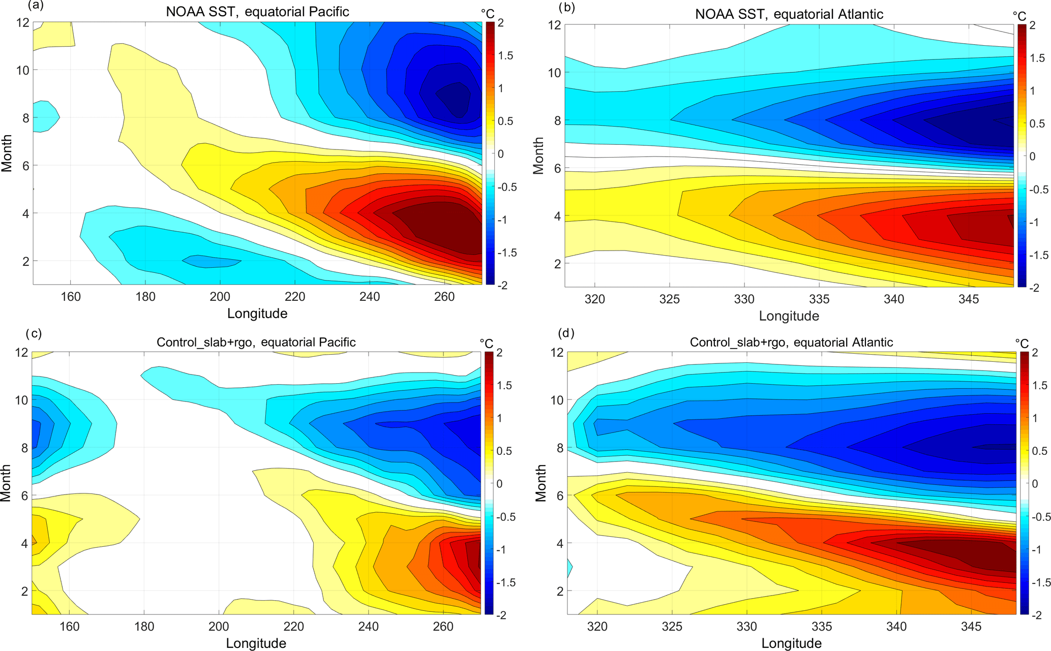
Figure 1(a, b) De-meaned SST seasonal cycle from NOAA SST data (Smith et al., 2008) in the equatorial Pacific (2∘ S–2∘ N, 150–270∘ E) and Atlantic (2∘ S–2∘ N, 320–345∘ E) respectively. (c, d) De-meaned SST seasonal cycle for Control_slab + rgo in the equatorial Pacific and Atlantic respectively. Contour interval: 0.2 ∘C.
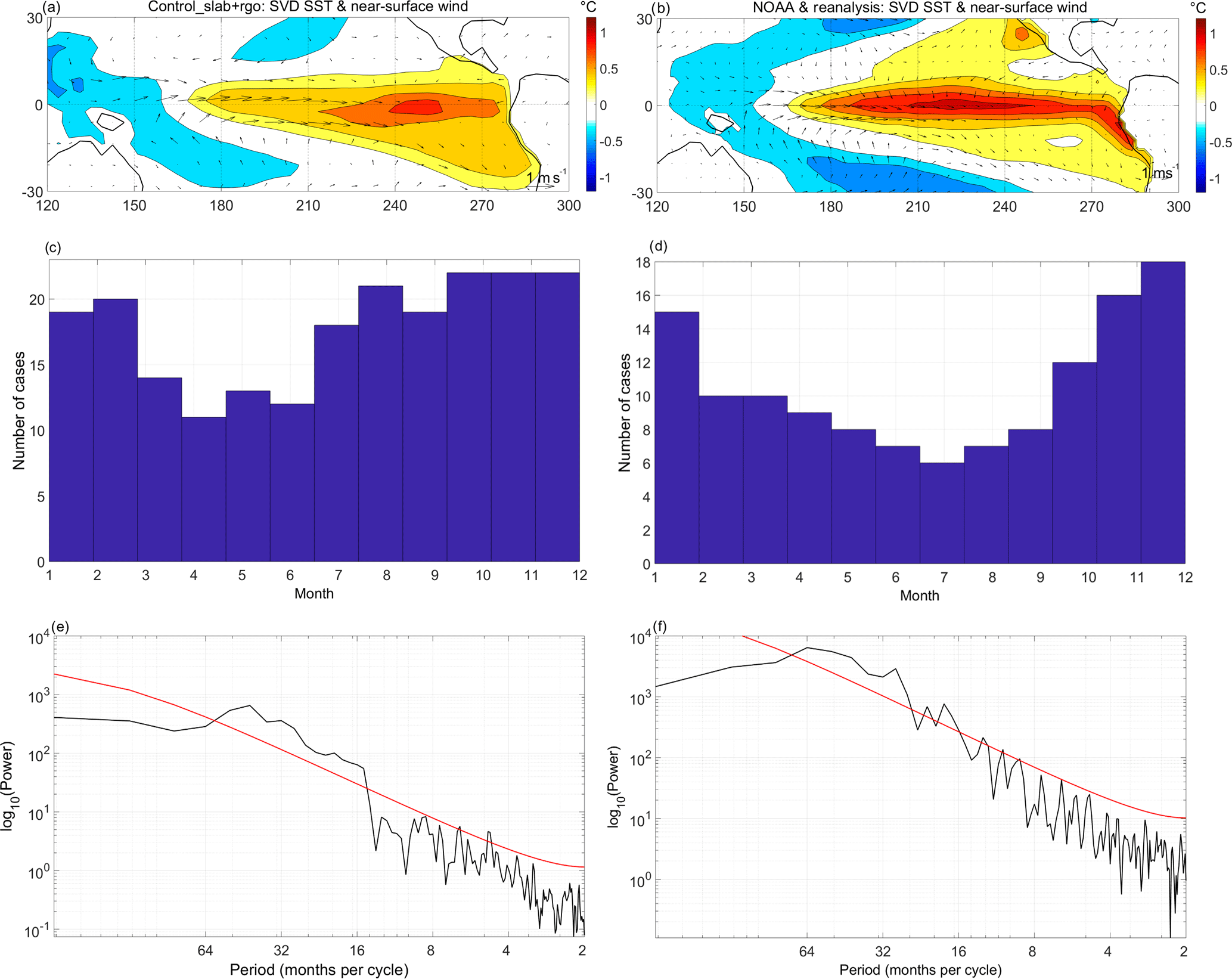
Figure 2First SVD pattern of SST and near-surface winds in the tropical Pacific Ocean (30∘ S–30∘ N, 120–300∘ E) for the Control_slab + rgo experiment (a, c, e) and NOAA SST and reanalysis data (b, d, g; Smith et al., 2008; Kalnay et al., 2006). (a, b) Spatial pattern; contour interval 0.2 ∘C. (c, d) Histogram showing phase-locking to the seasonal cycle. (e, f) Spectral analysis; the red line indicates the red-noise spectrum.
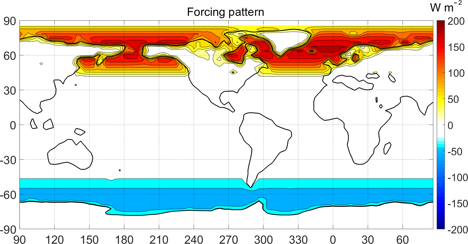
Figure 3Forcing pattern. The sign convention is positive out of sea. Contour interval 20 W m−2.
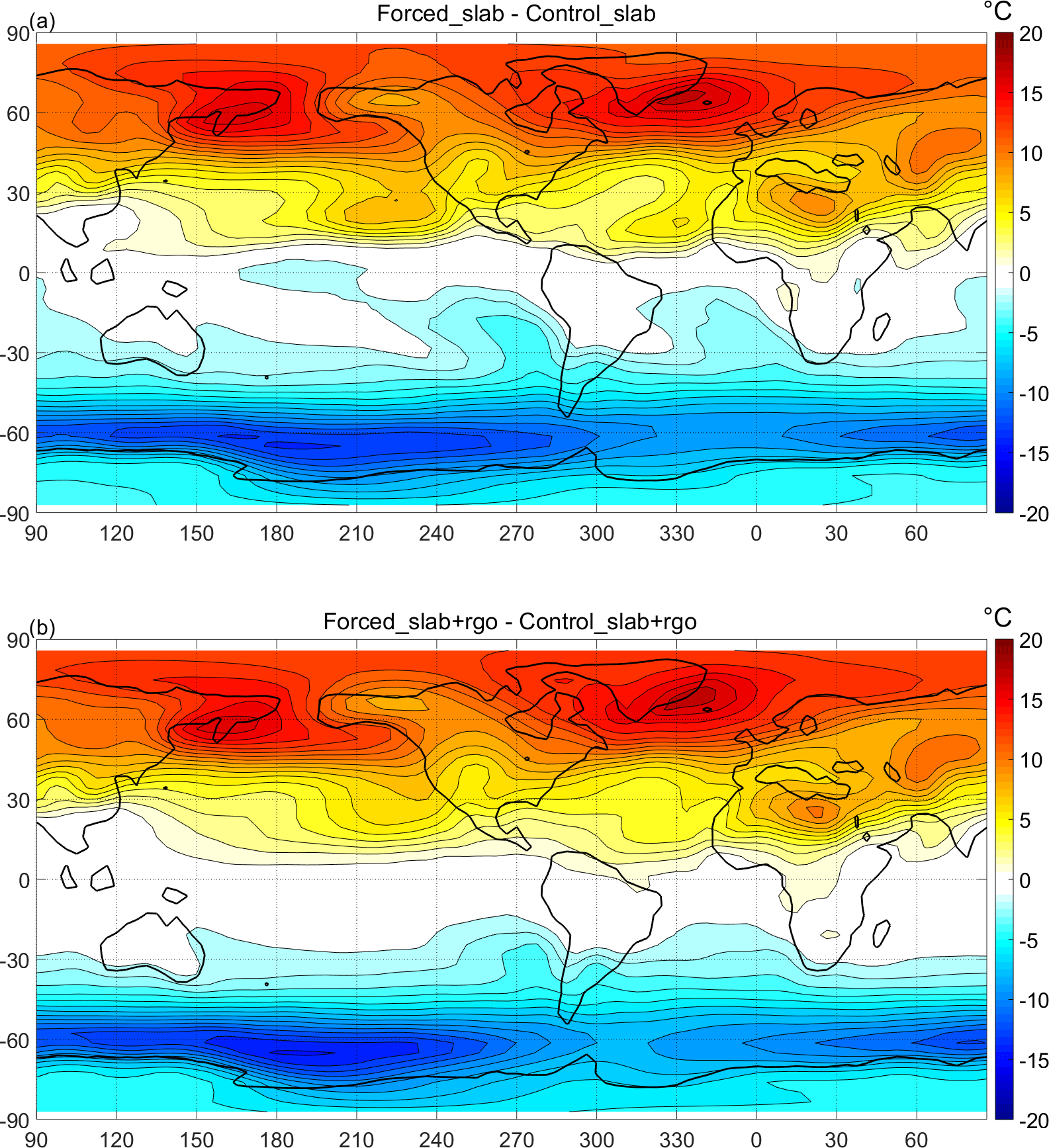
Figure 4Annual mean anomalies with respect to the control of NSAT for (a) Forced_slab and (b) Forced_slab + rgo. Contour interval 1 ∘C.
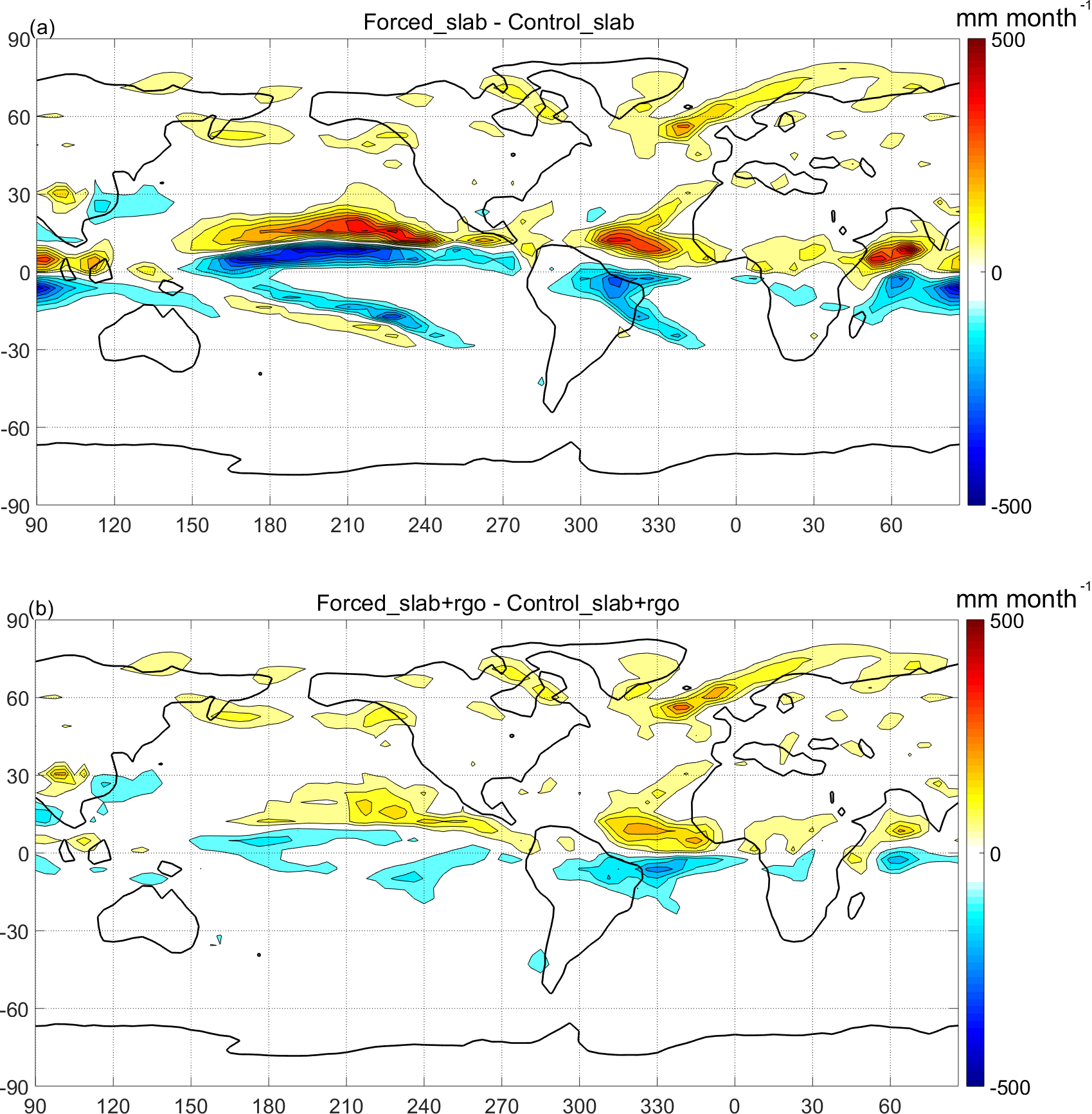
Figure 5Annual mean anomalies with respect to the control of precipitation for (a) Forced_slab and (b) Forced_slab + rgo. Contour interval 50 mm month−1.
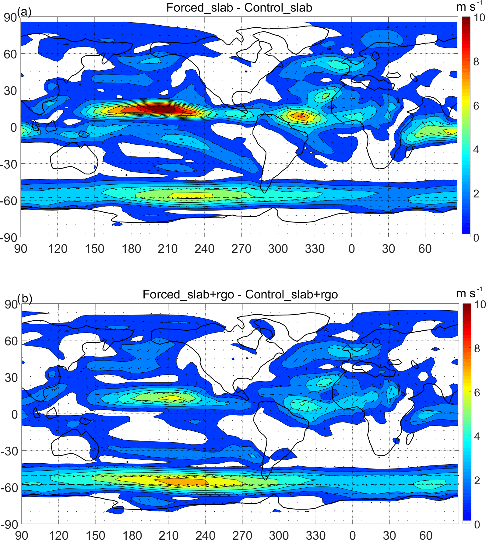
Figure 6Annual mean anomalies with respect to the control of near-surface (950 hPa) wind for (a) Forced_slab and (b) Forced_slab + rgo. Contour interval 1 m s−1.

Figure 7Northward atmospheric energy transport for the experiments: Control_slab, Control_slab + rgo, Forced_slab and Forced_slab + rgo.
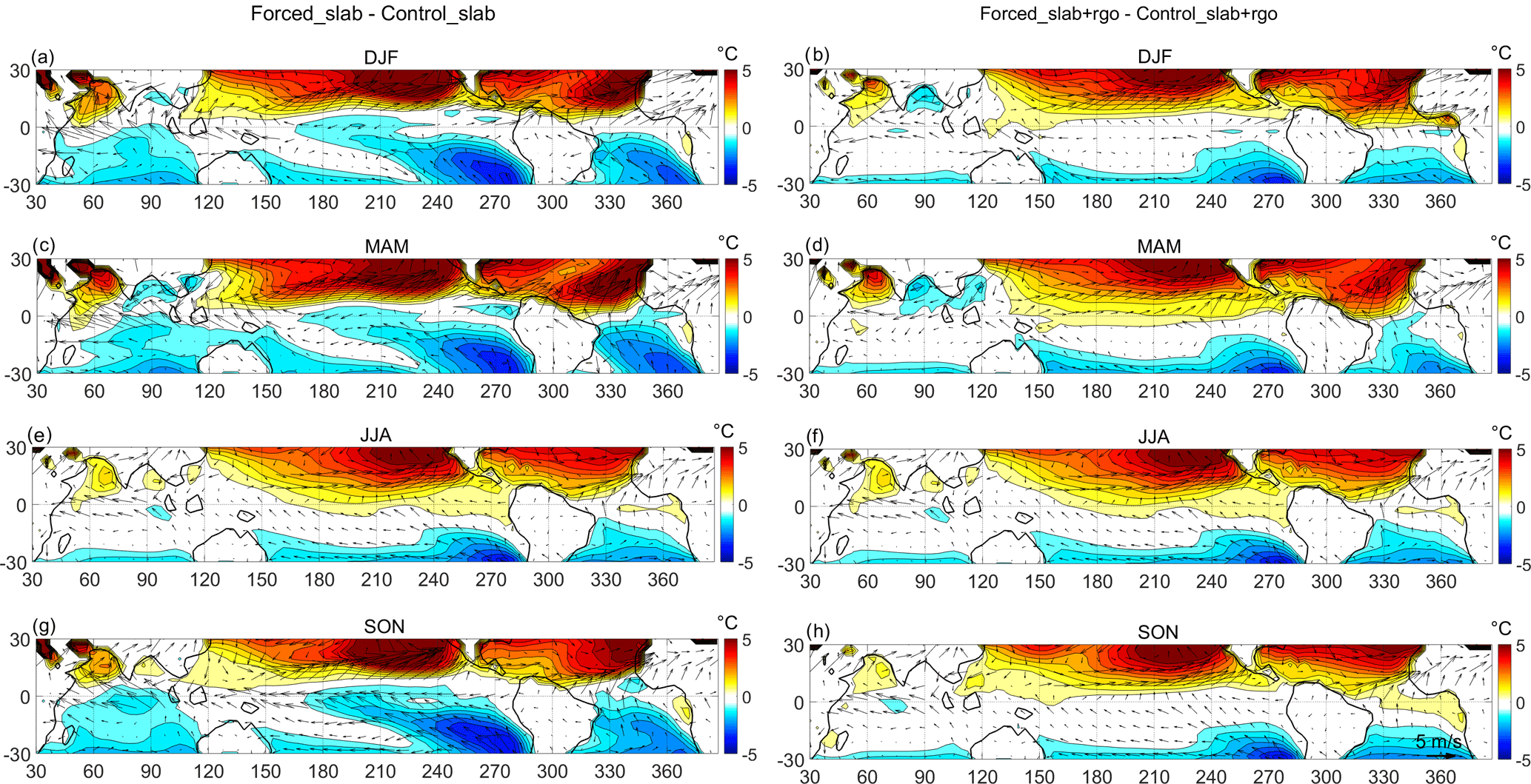
Figure 8Seasonal SST and near-surface wind anomalies with respect to the control for Forced_slab (a, c, e, g) and Forced_slab + rgo (b, d, f, h). (a, b) December–February; (c, d) March–May; (e, f) June–August; (g, h) September–November. Contour interval 0.5 ∘C.

Figure 9Equatorial Pacific Ocean (2∘ S–2∘ N, 150–270∘ E) de-meaned near-surface (950 hPa) zonal wind anomalies seasonal cycle for (a) Forced_slab and (b) Forced_slab + rgo experiments. Contour interval: 0.5 m s−1.

Figure 10Equatorial Pacific Ocean (2∘ S–2∘ N, 150–270∘ E) de-meaned SST anomalies seasonal cycle for (a) Forced_slab and (b) Forced_slab + rgo experiments. Contour interval: 0.2 ∘C.
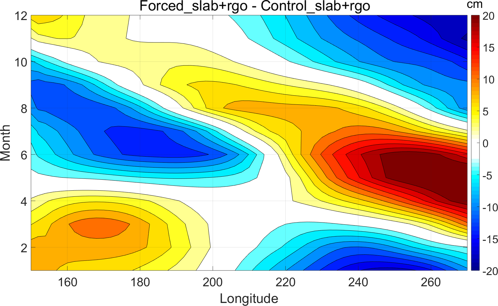
Figure 11Equatorial Pacific Ocean (2∘ S–2∘ N, 150–270∘ E) de-meaned thermocline depth anomalies seasonal cycle for the Forced_slab + rgo experiment. Contour interval: 2 cm.

Figure 12First SVD pattern of SST and near-surface winds in the tropical Pacific Ocean (30∘ S–30∘ N, 120–300∘ E) for the Forced_slab + rgo experiments. (a) Spatial pattern; contour interval 0.2 ∘C. (b) Histogram showing phase-locking to the seasonal cycle. (c) Spectral analysis; the red line indicates the red-noise spectrum.
Talento and Barreiro (2016) use an AGCM coupled to a slab ocean model to quantify the relative roles of the atmosphere, tropical sea surface temperatures (SSTs) and continental surface temperatures in the ITCZ response to extratropical thermal forcing. They find that if the tropical SSTs are not allowed to change, then the ITCZ response strongly weakens (although not negligible), particularly over the Atlantic Ocean and Africa. If, in addition, the land surface temperature over Africa is maintained the ITCZ response completely vanishes, indicating that the ITCZ response to the extratropical forcing is not possible just through purely atmospheric processes, but rather it needs the involvement of either the tropical SST or the continental surface temperatures. With the same model configuration, Talento and Barreiro (2017) focus on the South Atlantic convergence zone (SACZ) and show that, during its peak in austral summer, its response to warming in the NH extratropics and cooling in the SH extratropics consists of weakening, mostly due to the NH component of the forcing. Both studies showed strong changes in the tropical band where SST, surface winds and precipitation are strongly coupled. Nevertheless, in these studies important ocean dynamics are missing as the slab ocean can only simulate the thermodynamic exchange between the atmosphere and the ocean.
Chiang et al. (2008) explore the impact of an ITG on the tropical Pacific climate through simulations performed with an AGCM coupled to a medium-complexity ocean model: a reduced gravity ocean (RGO) model. They find that when the NH is warmer than the SH, the annual mean equatorial zonal SST gradient strengthens, associated with an earlier onset and a later retreat of the seasonal cold tongue together with an intensification during the peak cold season. They also find that El Niño–Southern Oscillation (ENSO) activity is sensitive to the ITG, with small ITG optimal for the development of ENSO activity.
Lee et al. (2015) also use an AGCM coupled to an RGO model and analyse the impact of the glacial continental ice sheet topography on the tropical Pacific climate. They suggest that the thickness of the ice sheets, separate from the ice albedo effect, has a considerable impact on the tropical climate. They identify two types of responses: a quasi-linear response directly associated with the topographic changes and a nonlinear response mediated through the tropical thermocline adjustment. They find that increasing the thickness of the continental ice sheets produces a southward displacement of the ITCZ and a weakening of the equatorial zonal SST gradient, caused by cooling (warming) in the western (eastern) equatorial Pacific, together with the thermocline deepening to the east. They note that the energy flux approach proposed in Kang et al. (2008, 2009) and Cvijanovic and Chiang (2013) does not appear to explain the ITCZ shifts in these experiments because even though the northern cross-equatorial energy transport increases with the ice thickness, the mid-latitude transport decreases.
Although most of the simulation studies on extratropical to tropical teleconnections focus on just one ocean model at a time, there is recent literature analysing the subject in a hierarchy of ocean model configurations.
Kay et al. (2016) study the effect of Southern Ocean cooling on the tropical precipitation, coupling an AGCM either to a slab or to a full oceanic model. They find that with dynamic ocean heat transport the tropical precipitation response is weaker with, in this case, most of the cross-equatorial heat transport carried out by the ocean and not by the atmosphere. Similar conclusions are obtained by Hawcroft et al. (2017) and Tomas et al. (2016) with different fully coupled models, suggesting that the results are not model specific. In the same direction, Green and Marshall (2017) perform a series of idealized simulations in aqua-planet mode with an AGCM coupled either to a dynamic or to a slab ocean model while an ITG is applied. They find that the oceanic circulation dampens the ITCZ shift in response to the ITG by a factor of 4 compared to the case when the ocean circulation is not allowed to respond to the forcing. They find that with a dynamic ocean the mechanical coupling of the tropical atmospheric and oceanic energy transport (through Ekman balance) ensures that the ocean circulation always transports energy across the Equator in the same direction as the atmosphere does, therefore helping offset the imposed thermal contrast and not requiring for the atmosphere to transport as much energy as when the ocean circulation is fixed.
From a theoretical perspective, Schneider (2017) confirms the simulation results and derives a quantitative framework that shows that the Ekman coupling of atmospheric and oceanic energy fluxes dampens the response of the ITCZ and calculates that, in the current climate in the zonal and annual mean, the factor of damping by Ekman coupling is of the order of 3.
To complement the results of the previously mentioned studies here we propose to analyse the tropical response to extratropical thermal forcing in a hierarchy of ocean model configurations, but by using an intermediate-complexity ocean model coupled only in the tropical oceans: an RGO model. These simulations, therefore, represent an additional and intermediate step into understanding the tropical ocean dynamics' role in the extratropical to tropical communication process.
The paper is organized as follows. In Sect. 2 we describe the models used, with special emphasis on the description of the RGO model and its validation against observational data. The experiments performed are explained in Sect. 3. The results can be found in Sect. 4, differentiated regarding changes in annual mean, seasonal cycle or ENSO. The summary and conclusions are presented in Sect. 5.
The atmospheric model used in this study is the Abdus Salam International Centre for Theoretical Physics (ICTP) AGCM (Molteni, 2003; Kucharski et al., 2006), which is a full atmospheric model with simplified physics. We use the model version 40 in its eight-layer configuration and T30 () horizontal resolution. The model includes parameterizations of: large-scale condensation, shallow and deep convection, shortwave radiation (using two spectral bands), longwave radiation (using four spectral bands), surface fluxes of momentum, heat and moisture and vertical diffusion. Present-day boundary surface conditions, orbital parameters and greenhouse forcing are used.
We analyse the outcomes of coupling the AGCM with two ocean models of different complexity. In the first configuration the AGCM is coupled with a slab ocean model; a monthly varying ocean heat flux correction (derived from a previous 30-year model integration with identical settings but with prescribed observed SSTs) is imposed in order to keep the simulated SST close to present-day conditions. In the second configuration, and in order to better reproduce the tropical ocean dynamics, an RGO model is coupled in the tropical region (30∘ S–30∘ N), while a slab ocean model is applied elsewhere. In this setup an annual-mean ocean heat flux correction is imposed in order to keep the simulated SST close to present-day conditions.
We proceed to describe the RGO model and to validate its results by comparison with observational analogous.
2.1 RGO model formulation and validation
We use an extension of the classical 1.5-layer RGO model, introduced by Cane (1979) to study the ENSO phenomenon. The extension of the model, as in Chang (1994), includes thermodynamics of the upper ocean and allows for the prediction of the SST.
The model consists of a 50 m depth upper layer in which mass, heat and momentum obey the conservation laws and a lower layer of infinite depth in which the velocity must be null so that the kinetic energy is finite. The approximation is reasonable for the tropical ocean because of the existence of a sharp thermocline which inhibits the downward propagation of waves generated in the upper ocean (Zebiak, 1985). To better predict changes of the SST, a linear and homogeneous frictional layer (assumed to concentrate most of the induced Ekman transport) is added to the model. The subsurface temperature is parameterized in terms of the thermocline depth, the observed annual mean temperature at 50 m depth (from Levitus, 1982) and the annual mean thermocline depth when the model is forced by observed wind stress.
The resolution of the RGO model is 1∘ in latitude and 2∘ in longitude, applied in the 30∘ S–30∘ N tropical band. The model is run using an anomaly coupling strategy. In this strategy, the oceanic and atmospheric components of the model exchange momentum and heat flux anomalies computed relative to their own model annual mean. The modelled anomalies are then superimposed on the observed annual mean. Sponge layers of 5∘ width are introduced at the northern and southern boundaries to eliminate artificial coastal Kelvin waves.
A 70-year control simulation in which the AGCM is coupled to the RGO in the tropics and to the slab ocean model elsewhere is produced. The last 50 years of the control run are used for averaging and comparison with observational analogues. We use the NOAA Extended Reconstructed SST V3b (Smith et al., 2008) and the near-surface winds from the NCEP/NCAR Reanalysis (Kalnay et al., 2006), for the period 1979–2013.
With the imposed heat flux correction, the annual mean SST in the control simulation strongly resembles the observed pattern (not shown). In addition, the model reasonably captures the main characteristics of the seasonal cycle in the equatorial (2∘ S–2∘ N) Pacific and Atlantic oceans (Fig. 1), although in the equatorial Pacific the de-meaned (annual mean removed) simulated SST seasonal cycle is weaker than in the observations. Also, the Pacific cold tongue is not well developed during SH summer.
The control simulation also reproduces the main mode of variability in the tropical Pacific Ocean quite realistically both in the spatial and temporal domains (Fig. 2; please note that in all the latitude–longitude maps in the manuscript the land and sea mask used by the model is the one depicted). The first coupled pattern arising from a singular value decomposition (SVD) of the monthly SST and surface wind characterizes ENSO and explains 81 % (62 %) of the variability in the observations (simulation). The simulated pattern is weaker than the observed, with the SST anomaly maximum located too far eastward. The phase-locking to the seasonal cycle of the simulated pattern peaks during the end of the calendar year as it does in the observations, but its distribution is more uniform throughout the year. Both simulated and observed spectra show statistically significant peaks relative to a red-noise null hypothesis from 16 to 60 months.
2.2 Experimental design
For each model configuration two runs are produced: a control run (in which no forcing is applied) and a forced run (in which extratropical forcing is imposed). The applied forcing pattern consists of cooling in one hemisphere and warming in the other poleward of 40∘, applied only over ocean grid points, and with a resulting global average forcing equal to zero. This pattern is similar to the one used in Kang et al. (2008) and in Talento and Barreiro (2016), and it is intended to represent the asymmetric temperature changes associated with glacial–interglacial and millennial-scale climate variability as well as the asymmetric SST pattern characteristic of the global warming trend. The forcing pattern is superimposed on a background state and is obtained as explained in Talento and Barreiro (2016).
The forcing pattern is shown in Fig. 3, in which sign convention is positive out of sea and, therefore, positive values of the forcing could be considered to represent a situation where the atmosphere is dry and colder than the ocean below it so that there is a strong ocean-to-atmosphere net heat flux. This forcing generates a near-surface temperature (NSAT) anomaly response of up to 16 ∘C (−20 ∘C) over the north Atlantic Ocean at 70∘ N (over the Ross Sea), as shown in Fig. 4. For comparison, in a climate simulation of the last 21 000 years (TRACE2k experiment, He, 2011) anomalies of about −10 ∘C (6 ∘C) are obtained over the North Atlantic (Antarctica) during Heinrich stadial 1, 18 000 to 15 000 years ago.
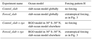
As mentioned before we use two ocean models. When the AGCM is coupled to a slab ocean model, the experiments are named Control_slab and Forced_slab. If an RGO is used in the tropical band while the slab ocean model is applied elsewhere, the corresponding experiments are named Control_slab + rgo and Forced_slab + rgo. In all the simulations the model was run for 70 years and the last 50 are used for averaging. Running the simulations for 70 years proved to be more than enough to reach the equilibrium; a timescale of 10 years was estimated to be the time span necessary for adjustment. In Table 1 we summarize the experiments. All the data are publicly available in Talento and Barreiro (2018).
First we analyse and compare the annual mean anomalies generated by the extratropical forcing with the two configurations implemented. Second, we will focus on the tropical Pacific climate and study the changes produced in the seasonal cycle for both setups. Finally, we will briefly investigate possible changes in ENSO activity when the RGO is coupled in the tropical oceans.
3.1 Annual means
In this subsection we compare the results obtained with the two implemented configurations in terms of annual means of different fields. The results are presented in the form of anomalies with respect to the corresponding control case.
Figure 4 shows the near-surface air temperature (NSAT) changes with respect to the corresponding control for the two configurations. In both experiments there is generalized warming (cooling) in the NH (SH), while in the southern tropics a strengthening of the zonal gradient is evident. The most pronounced differences between the two configurations are seen in the tropical region, in which the slab plus rgo configuration anomalies tend to be up to 1 ∘C weaker than the slab configuration anomalies. In particular, the equatorial Pacific cooling seen in the slab configuration is no longer present in the rgo + slab configuration, and the southeastern ocean basins do not cool as much. This suggests that, overall, tropical ocean dynamics tend to oppose changes in the annual mean conditions. In the extratropics the differences between the two configurations are barely noticeable, although regions of up to 2 ∘C are noted in the vicinity of the Antarctic Peninsula and Greenland.
As a consequence, tropical changes in precipitation are weaker when using the RGO: while in both experiments the most pronounced feature is a northward shift of the ITCZ, anomalies for the slab + rgo configuration are much weaker (Fig. 5). Also, in the slab configuration strong changes of tropical precipitation are found equally over the three ocean basins, but for the slab + rgo setup the most intense anomalies are seen over the Atlantic Ocean concurrent with a still relatively strong cross-equatorial SST gradient, suggesting a larger role for continental temperatures in controlling the position of the ITCZ (as in Talento and Barreiro, 2016). Changes in the subtropical convergence zones are also weaker in the slab + rgo configuration, differently from the southward shift seen in the slab configuration. In particular for the case of the South Atlantic convergence zone, this result is consistent with Talento and Barreiro (2016), which showed that during southern summer the weakening of the SACZ is related to the development of a region of strong rainfall in the tropical north Atlantic.
As expected from the above results, both experiments present similar patterns of near-surface (950 hPa) wind anomalies (Fig. 6): anomalous northward winds associated with the ITCZ northward displacement in the tropics, and anomalous westerly winds over the Southern Ocean. The Forced_slab + rgo response is weaker in the tropics but stronger over the Southern Ocean, compared to the Forced_slab response. Similar pictures of a weaker response in the case of slab + rgo configuration can be seen in upper-level winds, mean sea level pressure and mass stream-function (not shown).
To summarize, in Fig. 7 we present the northward atmospheric energy transport for the control and forced runs in the two configurations implemented. As can be seen, while the control runs display almost identical transport, the forced runs significantly disagree in magnitude in the tropical region, with the slab + rgo configuration producing the weakest changes with a decrease of the transport toward the southern high latitudes, representing damping by a factor of 1.9. In the perturbed runs, the energy flux equator is located around 12∘ N (8∘ N) for the slab (slab + RGO) configuration, equivalent to a damping in the shift by a factor of 1.5.
3.2 Seasonal cycle
As the previous subsection showed, the most pronounced differences between the two implemented configurations are found in the tropical band. Therefore, for the analysis of variations in the seasonal cycle we will focus on the 30∘ S–30∘ N region.
Three-month means of SST and near-surface wind changes for the tropics are shown in Fig. 8. In the Pacific Ocean, for the Forced_slab experiment negative SST anomalies are seen reaching the Equator (or even more to the north) in all four seasons, September–November (SON) being the period of strongest cooling and June–August (JJA) being the period in which the negative anomalies have the weakest penetration into the NH. Meanwhile, for the Forced_slab + rgo experiment the negative SST anomalies barely reach the Equator and, in fact, positive anomalies are the ones penetrating into the SH for the seasons March–May (MAM) and JJA. Consistent with these changes in response, the equatorial anomalous winds in the slab configuration are mainly easterlies throughout the year, while in the slab + rgo configuration they have a marked northward component and are eastward during MAM season. Also, the equatorial Atlantic tends to warm up during most of the year when using the RGO model.
Equatorial (2∘ S–2∘ N) de-meaned seasonal cycles for near-surface zonal wind and SST anomalies in the Pacific basin for the two experimental configurations are shown in Figs. 9 and 10 respectively. In Forced_slab there are eastward (westward) near-surface wind anomalies from December to May (June to November) distributed along the basin. The positive wind anomalies in the Forced_slab are quite uniform along the basin, although there are maximums in the western and eastern ends during December–February (DJF). The negative anomalies during the second half of the year are maximal in the central-eastern basin. In the slab configuration, the equatorial SST response to these wind anomalies is, however, very weak (Fig. 10a). On the other hand, when the RGO is coupled (and although the annual mean anomalies were even weaker than for the slab configuration; Fig. 4) there are substantial changes occurring to the seasonal cycle of SST in the central-eastern basin: from April to August (October to December) the forced run produces warming (cooling) of up to 1 ∘C (−0.8 ∘C). The location and timing of these anomalies lead to a substantial strengthening of the SST seasonal cycle in the eastern Pacific Ocean (overlap Fig. 10b on the Control_slab + rgo SST seasonal cycle shown in Fig. 1c).
The thermocline depth shows consistent changes when the RGO is used (Fig. 11): a deepening in the east of the basin starting around March and finishing in July, consistent with the warmer SSTs seen in the region (with 1-month lag). Considering the wind anomalies of the slab setup (Fig. 9a) as the forcing pattern for the ocean dynamics derived from the extratropical signal, this thermocline-deepening pulse appears to be initiated during the SH summer in the west of the basin (due to a weakening of the trades) and is propagated eastward as a Kelvin wave, reaching the eastern boundary 2–3 months later. The deepening of the eastern Pacific thermocline is concurrent with a shallowing in the western Pacific particularly from May to July, and vice versa (but less obvious) in other seasons of the year. In the second half of the year the strengthening of the trades locally shallows the thermocline in the eastern Pacific and the western Pacific recovers its mean depth.
In summary, the equatorial near-surface zonal wind changes caused by the extratropical forcing seen in the slab configuration induce dynamical ocean–atmosphere coupling that generates seasonal changes in the SST field when the RGO is used. This results in late austral autumn warming and cooling in spring and summer in the equatorial eastern Pacific, leading to a strengthening of the SST seasonal cycle with consistent changes in the thermocline depth.
3.3 ENSO
In this subsection we investigate how the interannual variability in the tropical Pacific is affected by the interhemispheric SST gradient induced by the imposed forcing.
The leading pattern of co-variability of SST and near-surface wind in the tropical Pacific basin when the extratropical forcing is applied is weaker than that obtained when no forcing is implemented (Figs. 12a and 2a), and it explains a smaller percentage of the total variability (46 % compared to 62 %). The phase-locking to the seasonal cycle (Figs. 12b and 2c) is also modified, being more uniformly distributed and with a peak season from July to the end of the calendar year. The frequency spectrum of the ENSO pattern under the effect of the extratropical forcing is characterized by shorter periods than in the absence of the forcing and has a peak at 24 months (Figs. 12c and 2e).
The weakening of the ENSO activity can be understood in relation to the changes produced by the extratropical forcing on the SST seasonal cycle in the eastern Pacific Ocean. According to the nonlinear frequency entrainment mechanism (Chang et al., 1994) ENSO amplitude is anticorrelated with the strength of the SST seasonal cycle. The frequency entrainment implies that a self-exciting oscillator (like ENSO) will give up its intrinsic mode of oscillation in the presence of strong external forcing (like a strong seasonal SST cycle) and acquire the frequency of the applied oscillating forcing. Therefore, in our case, as the extratropical forcing generates significant strengthening of the eastern Pacific SST seasonal cycle, a weakening of ENSO is expected according to this mechanism.
Assuming linear behaviour holds, our result of ENSO weakening is also in agreement with Timmermann et al. (2007). These authors analyse fully coupled GCMs in the context of an Atlantic meridional overturning circulation (AMOC) slowdown, producing generalized cooling of the NH and warming in the SH, and find that most of the models predict a ENSO intensification attributed to a seasonal cycle weakening. The weakening of ENSO activity in the presence of a northward ITG is also consistent with the work of Chiang et al. (2008), who use an AGCM coupled to an RGO model, a model configuration similar to ours. Although they do not attempt to explain the causes, they find that ENSO is sensitive to ITG with maximal activity when the ITG is close to zero and a weakened performance as the gradient increases in any direction.
We investigated and compared the response of the tropical climate to extratropical thermal forcing in a hierarchy of models in which an AGCM was coupled either to a simple slab ocean model (just thermodynamic coupling) globally or with a combination of an RGO model in the tropical oceans and a slab ocean model elsewhere.
First, we found that the two model configurations lead to considerably different climate responses. In particular, in tropical regions the signal produced in the RGO coupling case is weaker in terms of annual means, indicating that regional dynamical air–sea interaction opposes the remote signal. This result is in agreement with the quantitative framework proposed by Schneider (2017), who calculates an expression for the damping of the ITCZ shift in the case of atmosphere–ocean mechanical coupling. In addition, our result also agrees with the simulation experiments performed by Kay et al. (2016) and Green and Marshall (2017), who also obtained a weaker tropical response when using a fully coupled model than when the AGCM is only coupled to a slab model, therefore indicating that the ITCZ shift damping is also seen when an intermediate-complexity ocean model is coupled only in the tropics. In our experiments the energy flux equator (which can be regarded as an approximation for the ITCZ latitude) shift dampens by a factor of 1.5 in the case when tropical ocean dynamics are included, while the southward atmospheric energy transport experiences a damping by a factor of 1.9. In the simulations by Green and Marshall (2017) and in the quantitative work of Schneider (2017) the damping factors for the ITCZ shift were 4 and 3 respectively.
However, although the annual mean anomalies produced by the RGO setup are weaker, we find that the changes in the SST seasonal cycle are larger. In particular, over the equatorial Pacific Ocean, while the slab configuration produces no changes to the SST seasonal cycle, the RGO addition generates profound warming in the central-eastern basin from April to August balanced by cooling in the rest of the year, yielding almost null integration in the annual mean but also implying a significant strengthening of the seasonal cycle in the eastern Pacific. The response of the seasonal cycle to the imposed extratropical forcing is qualitatively similar to the one obtained by Chiang et al. (2008) in similar experiments, although in our case positive SST anomalies reach the eastern boundary of the basin preventing earlier onset of the seasonal cold tongue as found by these authors in their simulations. We hypothesize that the changes in the SST seasonal cycle are possible via the effect that the zonal wind stress has on the thermocline depth: the remote forcing produces positive anomalies of zonal wind stress to be exerted in the first half of the calendar year; in particular, the significant weakening of the trades over the western portion of the basin around February and March induces a thermocline-deepening pulse that propagates eastward in the form of a Kelvin wave, reaching the eastern boundary 2 months later, and generating warming of the SST over that region as a result. In the second half of the year stronger trades in the central-eastern basin shallow the thermocline producing local cooling of the SST. Since these mechanisms are not available under the slab configuration, the wind stress seasonal cycle changes are not able to produce any SST changes.
Finally, within the RGO setup, we briefly analysed possible changes in ENSO activity and found that under the effect of the extratropical forcing, considerable changes are produced in both the spatial and temporal domains with a weaker SST pattern and a time series that lacks low-frequency variability. We hypothesized that the weakening of the ENSO activity concurrent with the intensification of the SST seasonal cycle in the eastern equatorial Pacific Ocean could be due to the frequency entrainment mechanism. As future climate projections tend to agree on the fact that global warming will have an important northward ITG component (NH warming faster than the SH; Friedman et al., 2013), the possible sensitivity of ENSO to ITG is of utmost relevance. However, current state-of-the-art fully coupled climate models do not seem to agree on the projected future changes in ENSO characteristics, and no clear evidence for a correlation with ITG has been detected in future climate projections (Stevenson, 2012; Taschetto et al., 2014).
Data sets, codes and analysis scripts used in this study can be obtained from https://doi.org/10.17605/OSF.IO/ABRY8 (Talento and Barreiro, 2018).
The authors declare that they have no conflict of interest.
Part of this work was performed while the first author was supported by Universidad de la República, Agencia Nacional de
Investigación e Innovación (ANII, Uruguay) and the Belmont Forum and JPI-Climate Collaborative Research Action “INTEGRATE,
An integrated data-model study of interactions between tropical monsoons and extratropical climate variability and
extremes”. Comments by two anonymous reviewers are gratefully acknowledged.
Edited by: Ben Kravitz
Reviewed by: two anonymous referees
Broccoli, A. J., Dahl, K. A., and Stouffer, R. J.: Response of the ITCZ to Northern Hemisphere cooling, Geophys. Res. Lett., 33, L01702, https://doi.org/10.1029/2005GL024546, 2006.
Cane, M. A.: The response of an equatorial ocean to simple wind stress patterns. I-Model formulation and analytic results. II – Numerical results, J. Mar. Res., 37, 233–299, 1979.
Chang, P.: A study of the seasonal cycle of sea surface temperature in the tropical Pacific Ocean using reduced gravity models, J. Geophys. Res.-Oceans, 99, 7725–7741, 1994.
Chang, P., Wang, B., Li, T., and Ji, L.: Interactions between the seasonal cycle and the Southern Oscillation-Frequency entrainment and chaos in a coupled ocean–atmosphere model, Geophys. Res. Lett., 21, 2817–2820, 1994.
Chiang, J. C. and Bitz, C. M.: Influence of high latitude ice cover on the marine Intertropical Convergence Zone, Clim. Dynam., 25, 477–496, https://doi.org/10.1007/s00382-005-0040-5, 2005.
Chiang, J. C., Fang, Y., and Chang, P.: Interhemispheric thermal gradient and tropical Pacific climate, Geophys. Res. Lett., 35, L14704, https://doi.org/10.1029/2008GL034166, 2008.
Cvijanovic, I. and Chiang, J. C.: Global energy budget changes to high latitude North Atlantic cooling and the tropical ITCZ response, Clim. Dynam., 40, 1435–1452, 2013.
Folland, C. K., Palmer, T. N., and Parker, D. E.: Sahel rainfall and worldwide sea temperatures, 1901–85, Nature, 320, 602–607, https://doi.org/10.1038/320602a0, 1986.
Friedman, A. R., Hwang, Y. T., Chiang, J. C., and Frierson, D. M.: Interhemispheric temperature asymmetry over the twentieth century and in future projections, J. Climate, 26, 5419–5433, https://doi.org/10.1175/JCLI-D-12-00525.1, 2013.
Green, B. and Marshall, J.: Coupling of trade winds with ocean circulation damps ITCZ shifts, J. Climate, 30, 4395–4411, https://doi.org/10.1175/JCLI-D-16-0818.1, 2017.
Hawcroft, M., Haywood, J. M., Collins, M., Jones, A., Jones, A. C., and Stephens, G.: Southern Ocean albedo, inter-hemispheric energy transports and the double ITCZ: global impacts of biases in a coupled model, Clim. Dynam., 48, 2279–2295, 2017.
He, F.: Simulating Transient Climate Evolution of the Last Deglaciation with CCSM3, PhD Thesis, University of Wisconsin-Madison, http://www.cgd.ucar.edu/ccr/paleo/Notes/TRACE/he_phd_092010-1.pdf (last access: 16 March 2018), 2011.
Kalnay, E., Kanamitsu, M., Kistler, R., Collins, W., Deaven, D., Gandin, L., Iredell, M., Saha, S., White, G., Woollen, J., Zhu, Y., Chelliah, M., Ebisuzaki, W., Higgins, W., Janowiak, J., Mo, K. C., Ropelewski, C., Wang, J., Leetmaa, A., Reynolds, R., Jenne, R., and Joseph, D.: The NCEP/NCAR 40-Year Reanalysis Project. B. Am. Meteorol. Soc., 77, 437–472, https://doi.org/10.1175/1520-0477(1996)077<0437:TNYRP>2.0.CO;2, 1996.
Kang, S. M., Held, I. M., Frierson, D. M., and Zhao, M.: The response of the ITCZ to extratropical thermal forcing: idealized slab-ocean experiments with a GCM, J. Climate, 21, 3521–3532, https://doi.org/10.1175/2007JCLI2146.1, 2008.
Kang, S. M., Frierson, D. M., and Held, I. M.: The tropical response to extratropical thermal forcing in an idealized GCM: the importance of radiative feedbacks and convective parameterization. J. Atmos. Sci., 66, 2812–2827, https://doi.org/10.1175/2009JAS2924.1, 2009.
Kay, J. E., Wall, C., Yettella, V., Medeiros, B., Hannay, C., Caldwell, P., and Bitz, C.: Global climate impacts of fixing the Southern Ocean shortwave radiation bias in the Community Earth System Model (CESM), J. Climate, 29, 4617–4636, 2016.
Kucharski, F., Molteni, F., and Bracco, A.: Decadal interactions between the western tropical Pacific and the North Atlantic Oscillation, Clim. Dynam., 26, 79–91, https://doi.org/10.1007/s00382-005-0085-5, 2006.
Lee, S. Y., Chiang, J. C., and Chang, P.: Tropical Pacific response to continental ice sheet topography, Clim. Dynam., 44, 2429–2446, 2015.
Levitus, S.: Climatological atlas of the world ocean, NOAA Prof. Pap. 13, US Government Printing Office, Washington DC, 1982.
Molteni, F.: Atmospheric simulations using a GCM with simplified physical parametrizations. I: Model climatology and variability in multi-decadal experiments, Clim. Dynam., 20, 175–191, 2003.
Schneider, T.: Feedback of atmospheric ocean coupling on shifts of the intertropical convergence zone, Geophys. Res. Lett., 44, 11644–11653, https://doi.org/10.1002/2017GL075817, 2017.
Schneider, T., Bischoff, T., and Haug, G. H.: Migrations and dynamics of the intertropical convergence zone, Nature, 513, 45–53, 2014.
Smith, T. M., Reynolds, R. W., Peterson, T. C., and Lawrimore, J.: Improvements to NOAA's historical merged land-ocean surface temperature analysis (1880–2006), J. Climate, 21, 2283–2296, 2008.
Stevenson, S. L.: Significant changes to ENSO strength and impacts in the twenty-first century: results from CMIP5, Geophys. Res. Lett., 39, L17703, https://doi.org/10.1029/2012GL052759, 2012.
Talento, S. and Barreiro, M.: Simulated sensitivity of the tropical climate to extratropical thermal forcing: tropical SSTs and African land surface, Clim. Dynam., 47, 1091–1110, https://doi.org/10.1007/s00382-015-2890-9, 2016.
Talento, S. and Barreiro, M.: Control of the South Atlantic Convergence Zone by extratropical thermal forcing, Clim. Dynam., 50, 885–900, https://doi.org/10.1007/s00382-017-3647-4, 2017.
Talento, S. and Barreiro, M.: Data: Sensitivity of the tropical climate to an interhemispheric thermal gradient: the role of tropical ocean dynamics, https://doi.org/10.17605/OSF.IO/ABRY8, 2018.
Taschetto, A. S., Gupta, A. S., Jourdain, N. C., Santoso, A., Ummenhofer, C. C., and England, M. H.: Cold tongue and warm pool ENSO events in CMIP5: mean state and future projections, J. Climate, 27, 2861–2885, https://doi.org/10.1175/JCLI-D-13-00437.1, 2014.
Timmermann, A., Okumura, Y., An, S.-I., Clement, A., Dong, B., Guilyardi, E., Hu, A., Jungclaus, J. H., Renold, M., Stocker, T. F., Stouffer, R. J., Sutton, R., Xie, S.-P., and Yin, J.: The influence of a weakening of the Atlantic meridional overturning circulation on ENSO, J. Climate, 20, 4899–4919, 2007.
Tomas, R. A., Deser, C., and Sun, L.: The role of ocean heat transport in the global climate response to projected Arctic sea ice loss, J. Climate, 29, 6841–6859, https://doi.org/10.1175/JCLI-D-15-0651.1, 2016.
Wang, X., Auler, A. S., Edwards, R. L., Cheng, H., Cristalli, P. S., Smart, P. L., Richards, D. A., and Shen, C. C.: Wet periods in northeastern Brazil over the past 210 kyr linked to distant climate anomalies, Nature, 432, 740–743, https://doi.org/10.1038/nature03067, 2004.
Zebiak, S. E.: Tropical atmosphere-ocean interaction and the El Niño/Southern Oscillation Phenomenon, PhD Thesis, Massachusetts Institute of Technology, Dept. of Earth, Atmospheric, and Planetary Sciences, 1985.