the Creative Commons Attribution 4.0 License.
the Creative Commons Attribution 4.0 License.
 | 06 Nov 2018
Cascading transitions in the climate system
Mark M. Dekker
Anna S. von der Heydt
Henk A. Dijkstra
We introduce a framework of cascading tipping, i.e. a sequence of abrupt transitions occurring because a transition in one subsystem changes the background conditions for another subsystem. A mathematical framework of elementary deterministic cascading tipping points in autonomous dynamical systems is presented containing the double-fold, fold–Hopf, Hopf–fold and double-Hopf as the most generic cases. Statistical indicators which can be used as early warning indicators of cascading tipping events in stochastic, non-stationary systems are suggested. The concept of cascading tipping is illustrated through a conceptual model of the coupled North Atlantic Ocean – El Niño–Southern Oscillation (ENSO) system, demonstrating the possibility of such cascading events in the climate system.


Earth's climate system consists of several subsystems, e.g. the ocean, the atmosphere, ice and land, which are coupled through fluxes of momentum, mass and heat. Each of these subsystems is characterized by specific processes, on very different timescales, determining the evolution of its observables. For example, processes in the atmosphere occur on much smaller timescales than in the ocean; hence, in weather prediction the upper ocean sets the background state for the evolution of the atmosphere. Similarly, in equatorial ocean–atmosphere dynamics associated with the El Niño–Southern Oscillation (ENSO) phenomenon, the global meridional overturning circulation can be considered a background state, as it evolves on a much larger timescale.
This notion that one subsystem provides a background state for the evolution of another subsystem is important when critical transitions are considered. In the climate system, a number of tipping elements have been identified (Lenton et al., 2008 give an overview of these), where changes in observables can occur relatively rapidly compared to the changes in their forcing near so-called “tipping points”. Examples of tipping elements are the Atlantic meridional overturning circulation (AMOC) (Stommel, 1961), the Arctic sea ice (Bathiany et al., 2016), monsoon patterns, mid-latitude atmospheric flow (Barriopedro et al., 2006), vegetation cover (Hirota et al., 2011) and more local systems like coral reefs and permafrost. When one subsystem undergoes a transition, which changes the background state of another subsystem, a transition may also be induced in that second subsystem. Such dynamical interactions which lead to coupled transitions are examples of “tipping cascades” or “domino effects” (Kriegler et al., 2009; Lenton and Williams, 2013).
Many tipping points have been analysed in separate subsystems, both for phenomena of the present-day climate (Bathiany et al., 2016; Lenton, 2011), and for past climates (such as the abrupt cooling of the Younger Dryas, Livina and Lenton, 2007, and the desertification of the Sahel region, Kutzbach et al., 1996). However, less attention has been paid to the interaction between transitions in different subsystems. For example, when the AMOC collapses, precipitation patterns may change such that the equilibrium structure of the vegetation cover in the Amazon rainforest is shifted (Aleina et al., 2013). This may result in another transition, concerned with forest growth or dieback. Another example is the influence of the AMOC on the trade winds (through meridional sea surface temperature gradients), which in turn influence the amplitude of ENSO. In models, a collapse of the AMOC has been found to intensify ENSO (Dong and Sutton, 2007; Lenton and Williams, 2013; Timmermann et al., 2007), although there are also other effects that would weaken ENSO (Timmermann et al., 2005).
An example in past climates is the coupling between the ocean's overturning circulation and land ice. The rapid glaciation of the Antarctic continent around the Eocene–Oligocene boundary (34 Ma) is often explained in terms of a CO2 threshold being reached that allowed a major ice sheet to grow (DeConto and Pollard, 2003; Gasson et al., 2014). However, a two-step signal is found in the oxygen isotopic ratio, δ18O, which is attributed to a deep-sea temperature drop followed by the (slower) growth of the Antarctic Ice Sheet (AIS). One suggestion to explain the two-step transition is that the deep-sea temperature drop was related to a change in the pattern of the global MOC (Tigchelaar et al., 2011). The ice sheet formation is then argued to have been driven by decreasing atmospheric CO2 (Pearson et al., 2009). The switch in MOC (first tipping) led to the changes in the atmospheric CO2 (e.g. Elsworth et al., 2017) which caused the growth of the AIS (second tipping). This leads to the question of whether a cascading tipping event occurred.
In the last few years, much work has been carried out to formulate statistical indicators and early warning signals of tipping points. A system close to a critical transition shows features of a “critical slowing down” (Dakos et al., 2008; Kuehn, 2011; Scheffer et al., 2009). In the vicinity of the tipping point, the system slowly loses its ability to recover from small perturbations. This results in increased variance, auto-correlation and potentially also increased skewness and flickering (Scheffer et al., 2009). Various methods providing a specific scalar and a threshold when approaching the transition have been suggested, such as degenerate fingerprinting (Held and Kleinen, 2004; Thompson and Sieber, 2011) and detrended fluctuation analysis (DFA) (Livina and Lenton, 2007; Peng et al., 1994).
When considering cascading tipping points, the auto-correlation of two time series and their interaction need to be analysed simultaneously. Podnobik and Stanley (2008) proposed an altered form of DFA to assess the cross-correlation between two non-stationary time series and called this method detrended cross-correlation analysis (DCCA). In the computation of the fluctuation function, they used cross-covariance instead of auto-covariance and fit this to a power law. This concept is further extended by defining a coefficient ρDCCA that accounts for the auto-covariance of the individual time series (Yuan et al., 2015; Zhou, 2008). However, no statistical analysis or indicators have yet been formulated for cascading tipping events.
In this paper, we provide a quantitative approach to cascading tipping events. We start with a mathematical framework to formulate elementary cascading tipping points (Sect. 2). Next, we discuss statistical metrics to analyse, diagnose and potentially predict cascading transitions, and apply them to ensemble simulations of the elementary cascading tipping points (Sect. 3). Finally, we apply the new concepts to an example within the climate system: the potential cascading tipping mechanism between the AMOC and ENSO (Sect. 4). We summarize and discuss our findings in Sect. 5.
In the climate system, tipping points are usually related to rapid transitions, where an observable in the climate system may change abruptly in a relatively short time compared with changes in the forcing of the observable. Such rapid changes usually involve transitions from one equilibrium state to another, which can often be explained using classical bifurcation theory for autonomous dynamical systems. To a certain extent, these concepts can also be applied to non-autonomous systems (so-called slow–fast systems) when the time variation of parameters can be viewed as a slow external forcing (Kuehn, 2011). They form the basics for understanding phenomena such as noise-induced tipping (Thompson and Sieber, 2011) and rate-dependent tipping (Ashwin et al., 2012).
In this section, we present a mathematical framework for simple cascading transitions, which acts as a first step towards analysing the more complex real-world transitions. We focus on bifurcation-induced tipping points, and consider two types of bifurcations that are thought to be relevant to mechanisms of abrupt changes in the climate system; the back-to-back saddle-node bifurcation is often used to explain transitions between two coexisting equilibria (multi-stable systems), while the Hopf bifurcation can explain the appearance of oscillatory behaviour (Thompson and Stewart, 2002). Therefore, abrupt change in the system appears as a consequence of a parameter crossing a specific critical value at the bifurcation point.
A back-to-back saddle-node bifurcation (two saddle-nodes connected by a common unstable branch) generically occurs in physical systems (that have bounded states) when one parameter varies and the simplest dynamical system has a bifurcation that is described by
where the ai () are constants, ϕ is a parameter, x is the state variable and t is time. There are multiple equilibria in the system if and only if a1<0, a2>0 and within the parameter interval . In this case, the back-to-back saddle-node bifurcations occur at . In the following, we often use the terms “fold bifurcation” and “saddle-node bifurcation”, although in practise we only use “back-to-back” saddle-node bifurcations.
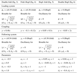
Table 1Parameter values and coupling for the four types of cascading tipping as shown in Figs. 1 and 2.
A Hopf bifurcation also generically occurs in physical systems, and the simplest dynamical system in which it occurs when one parameter is varied is described by
where, again, are constants, ϕ is the parameter, (x, y) is the state vector and t is time. The state vector satisfying (Eq. 2) reaches a stable periodic orbit if and only if a1b1<0 and ϕ>0; the transition from steady to periodic occurs at ϕ=0.
There are two other bifurcations when one parameter is varied (the transcritical and pitchfork bifurcations); however, these bifurcations are non-generic because special conditions must hold (e.g. symmetry) and so they are not considered here. Using the saddle-node and Hopf bifurcations, cascading tipping can be viewed as a combination of two coupled subsystems, where each subsystem undergoes one of these two types of bifurcations. Combining these bifurcations leads to four types of cascading tipping, which are discussed in the following.
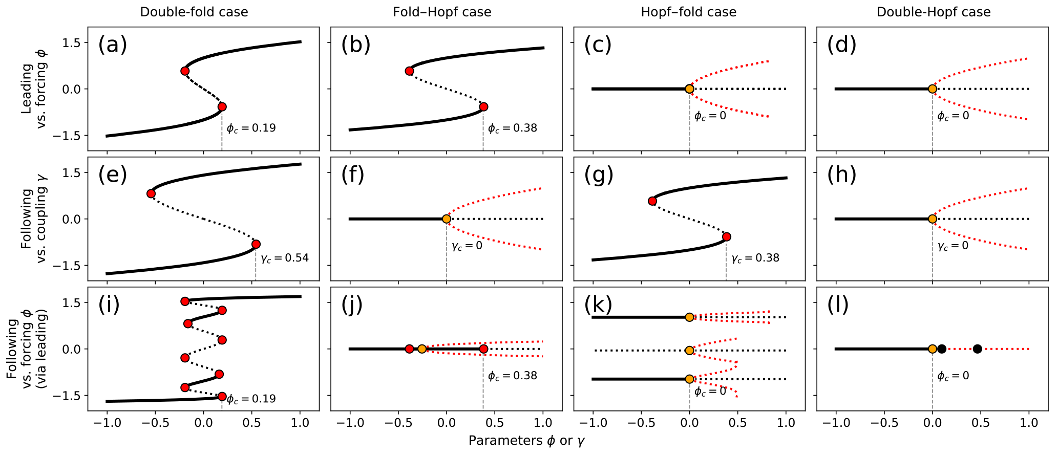
Figure 1Stable (solid), unstable (black dotted) and oscillatory (amplitude red dotted) regimes of various cascading tipping types (as defined on top of the figure). Red, orange and black dots indicate fold, Hopf and torus bifurcations, respectively. Leading system versus forcing ϕ (a–d). Following system versus coupling γ (e–h). Following system versus forcing ϕ (via leading) (i–l). Critical values of (coming from lower branch) leading tipping (a–d), following tipping (e–h) and the combined cascading tipping event (i–l) are marked by the grey vertical dashed line.
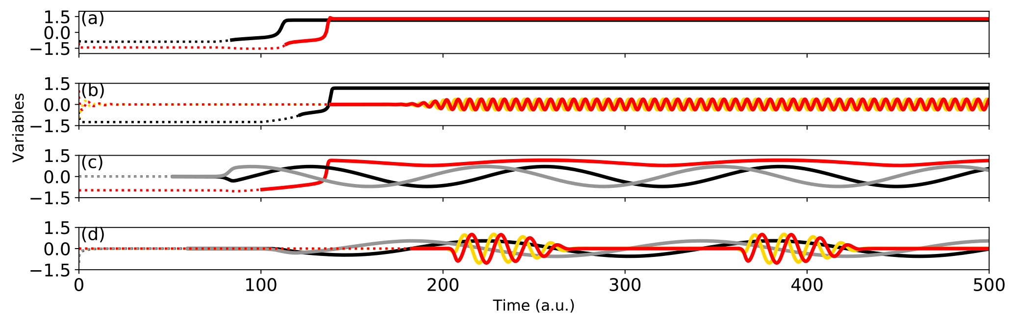
Figure 2 Example simulations for each cascading event type: the double-fold cascade (a), the fold–Hopf cascade (b), the Hopf–fold cascade (c) and the double Hopf cascade (d). Black and grey lines indicate the leading systems, red and yellow lines indicate the following systems. Dotted lines indicate time before the critical threshold in the forcing ϕ(t) (black/grey) or coupling κ(x) (red/yellow) is reached, solid lines indicate the time after this. Parameter values for the modelled systems are given in Table 1.
Coupling two systems introduces a direction to the cascade and we take account of this by defining a “leading” system, which during its transition changes a parameter (that is, the coupling term) in the “following” system. The changing parameter in the following system can then bring the following system closer to a bifurcation point, potentially even resulting in a second transition. In this section, we only look at deterministic cases, which do not allow for noise to play a role in the tipping. Therefore, transitions in the leading system result in a changed coupling term that can lead to transitions in the following system. In bifurcation diagrams versus forcing, the bifurcation points (for deterministic systems) can overlap. However, the transitions are distinguishable in transients, because the following system always tips after the completion of the first transition. This is why we show the bifurcation diagrams of both systems versus forcing (Fig. 1) and an example of a transient (Fig. 2) for each type. They will be discussed in more detail below.
2.1 Double-fold cascade
The most intuitive system that has the potential to undergo a cascading tipping event is a system where both the leading and the following system have saddle-node bifurcations. Analogous to Eq. (1), a dynamical system containing a double fold cascade is then
where x is the state vector of the leading system, y is the state vector of the following system, ai,bi () are constants, and ϕ is a parameter in the leading system. The key here is that the function γ, which serves as a parameter in the following system, depends on the leading system. The most simple coupling between the two systems is represented by . Observe that a change in the forcing parameter ϕ can induce a transition in x, which may affect the coupling function γ such that y also undergoes a transition. We would like to emphasize that the forcing ϕ does not directly affect y, and that y is only affected through a change in x (which is effectively only significant when x tips).
Implementing this system with the values shown in Table 1 gives insight in the system's equilibrium structure (Fig. 1a) and transient behaviour (example in Fig. 2a). When ϕ is changed moving through the bistable regime of the leading system the coupling moves the following system through its own bistable regime (see Table 1). Figure 1a and b show the equilibria of the leading (versus ϕ) and following systems (versus γ), respectively, showing the bistable regime in the centre of the figure, embedded in the saddle-node structure. Varying ϕ alters the state of the leading system, which affects the state of the following system through the coupling γ. This results in the existence of four stable states in the following system of the bistable regime of the leading system: two per state of the leading system, as shown in Fig. 1i. The leading system's state acts as a background condition modulating the position of the following system's equilibria; therefore, in case of transition, the leading system's state may drastically reposition the equilibria of the following system. This is intuitively visible in Fig. 2a, where a time series example of the dynamical system in Eq. (3) shows a cascading tipping event (parameters shown in Table 1). When the leading system (black) is forced (by changing ϕ) to move from a bistable to a monostable regime, it transits towards a new equilibrium. During this transition, the following system (red) is affected and leaves the regime in which it had four possible equilibria; it also transits to a different state.
2.2 Fold–Hopf cascade
The second type of cascading tipping event involves a saddle-node bifurcation in the leading system and a subsequent Hopf bifurcation in the following system. Using analogous notation as in Eq. (3), the simplest system that captures this so-called fold–Hopf cascade is
where x is again the state vector of the leading system, and (y, z) is the state vector of the following system. By slowly varying the parameter ϕ (e.g. linearly as ϕ(t)) the leading system moves through its bistable regime (see Table 1 for parameter values) and via the coupling forces the following system across the Hopf bifurcation point.
The bifurcation structure of the leading system of Eq. (4), using the parameters stated in Table 1, is displayed in Fig. 1b. As in Fig. 1a, this system's bifurcation diagram shows a saddle-node structure. The following system in Fig. 1f, now undergoes a Hopf bifurcation and subsequent oscillatory behaviour. In Fig. 1j, it can be seen that increasing ϕ on the lower branch of the leading system regime will still result in a stationary equilibrium for the following system. When increasing ϕ across ϕc, the leading system moves towards another state (seen in Fig. 1b) and the coupling γ increases (across γc in Fig. 1f). An oscillation then occurs in the following system. This mechanism makes it possible for steady and oscillatory states to coexist on the right side of the Hopf bifurcation in Fig. 1j. An example of a time series showing a fold–Hopf cascading event is displayed in Fig. 2b. A transition in the leading system (black) brings the following system (red/yellow) into an unstable equilibrium that eventually leads to an oscillatory state.
2.3 Hopf–fold cascade
A third type of cascading event involves a Hopf bifurcation in the leading system and a subsequent saddle-node bifurcation in the following system. Using similar notation to the previous subsection, the simplest system with a Hopf–fold cascade (see Table 1 for parameter values) is given by
where (x, y) is the state vector of the leading system, and z is the state vector of the following system. Again, we can slowly increase ϕ so that the leading system (x, y) crosses a Hopf bifurcation; via the coupling the following system is then moved through its bistable regime and a fold is reached in z.
Figure 1c contains the typical bifurcation structure of the leading system in Eq. (5), containing a Hopf bifurcation separating a stationary from an oscillatory regime. The following system's equilibrium structure for varying γ is given by Fig. 1g. In this particular configuration, for any negative ϕ there are multiple stable equilibria, as seen in Fig. 1k. This makes sense, as ϕ only affects the following system via its impact on the leading system, and for negative ϕ the leading system remains constant. At ϕ=0, the Hopf bifurcation in the leading system is reached and (x, y) starts oscillating. The following system oscillates a little along with the leading system due to the oscillatory changing value of γ.
When ϕ increases more, the amplitude of the leading system's oscillation grows, which eventually causes γ to cross the threshold; the following system then leaves its bistable regime (be it temporarily as γ will be reduced again due to the oscillation). This forces the following system into its upper branch, as can be seen in Fig. 1g. The upper branch's stable oscillation ends at ϕ≈0.8 (in Fig. 1k), because the amplitude becomes large enough for the system to swap between multiple equilibria. An example of such a cascading transition event can be seen in Fig. 2c, where an oscillation starts in the leading system (black/grey). A particular phase of this oscillation then causes the following system (red) to transit into the second equilibrium.
2.4 Double-Hopf cascade
A fourth type of cascading tipping event discussed here involves a Hopf bifurcation in the leading system and a subsequent Hopf bifurcation in the following system. Using analogous notation to the previous subsections, this double Hopf cascade is captured by the following dynamical system:
where (x, y) is the state vector of the leading system, and (u, v) is the state vector of the following system. If ϕ forces (x, y) such that it crosses the Hopf bifurcation point, the coupling causes a crossing of the second Hopf bifurcation in (u, v).
Figure 1d and h show the bifurcation diagrams of the leading and following systems, with supercritical Hopf bifurcations. The following system (in Fig. 1l) is stationary for many values of ϕ, up to the point that the leading system starts oscillating, which for high enough values of ϕ is large enough to make the following system cross the Hopf bifurcation. However, γ oscillates with the leading system (for ϕ>0). This means that oscillatory behaviour in the following system can only be expected in a particular part of the leading system's oscillation period. This interaction between the two oscillations result in torus bifurcations for particular values of ϕ. An example of a time series showing a double-Hopf cascading transition is shown in Fig. 2d. After a (slow) oscillation in the leading system (black/grey) has started, a (fast) oscillation in the following system (red/yellow) arises in particular phases of the slow oscillation.
In the previous section we formulated elementary deterministic dynamical systems that can exhibit cascading tipping. In order to detect tipping events from, for example, observed time series in real systems, we need to detect whether a system is close to a critical transition. In general, systems close to critical transition recover more slowly from perturbations, which in turn increases memory in the time series. This leads to the phenomenon of “critical slowing down” prior to bifurcation points. In this section, we simulate cascading tipping events to (a) study the statistical character of such events, (b) diagnose (post-tipping) whether tipping events are causally related and (c) take a first step towards statistical indicators for the prediction of cascading tipping events.
3.1 Methods for single tipping points
Several methods have been suggested for the analysis of time series to detect the approach of a single tipping point. For saddle-node bifurcations, the key features of a time series such as this is a critical slowing down. This can be investigated using standard quantities such as increasing auto-correlation (e.g. the lag-1 auto-correlation), increasing variance and increasing skewness (Held and Kleinen, 2004; Kuehn, 2011; Scheffer et al., 2009). Although critical slowing down near critical transitions is a general feature of (even chaotic) dynamical systems (Tantet et al., 2018), the standard metrics like auto-correlation at lag 1 and variance do not always provide an early warning signal (e.g. in Greenland ice core data in Livina and Lenton, 2007). Hence, more complicated indicators have been introduced, such as (i) degenerate fingerprinting (DF) and (ii) the detrended fluctuation analysis (DFA) (Held and Kleinen, 2004; Livina and Lenton, 2007; Peng et al., 1994; Thompson and Sieber, 2011). DFA is argued to be a solution to the problem that the simple lag-1 auto-correlation does not capture the approach to a transition in highly non-stationary data in long time series (Livina and Lenton, 2007; Peng et al., 1994). The latter is characterized by high auto-correlation due to the gradual increase or decrease of the system itself, distorting the signal of the critical slowing down, a problem in standard metrics and DF.
As critical slowing down implies an increasing auto-regressive behaviour in the time series prior to a transition, the memory component is increased. In general, the first step in DF is the projection of the data fields onto the leading EOF, which gives a time series xn (Held and Kleinen, 2004). After time-equidistant interpolation and detrending of the data, in the DF method one fits the following general auto-regressive process to the time series xn:
where ηn is Gaussian white noise and is the AR(1) coefficient. Here λ can be seen as the decay rate of perturbations in previous time steps. As the approaching of a bifurcation point involves an increase in memory, the value of c is presumed to increase towards one when approaching a saddle-node bifurcation point.
In DFA, one first chooses an integer window size s and divides the (cumulative-summed) time series X(n) into segments that do not overlap, where N is the length of the time series. In every window, the best polynomial fit of a chosen order is calculated. A quadratic polynomial is used here. The squared deviation from this quadratic polynomial for every window is summed, resulting in a measure of the auto-covariance fluctuating around the fit:
where X is the detrended time series and xν is the best polynomial fit in segment ν. Next, an average is taken over all segments to obtain the fluctuation function F(s):
which depends solely on s. The long-range auto-correlations can now be recognized by fitting the fluctuation function to a power law and looking at the resulting DFA-exponent α, according to
For α≤0.5, there is no long-term correlation and the fluctuations are indistinguishable from white noise. However, when α>0.5, there are long-term correlations present and for α≥1.5 the system has reached a bifurcation point. In the simulations analysed here the DFA scaling exponent is fitted explicitly for every (moving) window.
3.2 Methods for cascading tipping points
Cascading tipping involves two systems with their own bifurcation structure and their proximity towards bifurcation points. Although the leading system may be close to tipping, the following system might still be far from its bifurcation point and needs the critical transition of the leading system to even come close to this point; this makes the behaviour of the following system more prone to noise, less dependent on the leading system and less auto-correlated prior to the first tipping. This is why the general measures for single tipping events cannot be used, nor can regular cross (Pearson) correlation. The reason for this is that the following and leading systems do not have a one-to-one relationship (that is, weakly Pearson correlated), but are rather coupled through specific parameters, which is only visible in long-range correlations.
When approaching a cascading tipping point, the long-range cross-correlation between the leading state x and the following state y is expected to increase. The state x becomes more auto-correlated and is less susceptible to noise, and therefore influences y through the coupling in a more robust way. To find long-range cross-correlations, the so-called “detrended cross-correlation analysis” (DCCA) method was developed (Podnobik and Stanley, 2008; Zebende, 2011; Zhang et al., 2001; Zhou, 2008). Instead of using the auto-covariance to calculate the fluctuation function, as is used in Eq. (8), one uses the cross-covariance as follows:
The symbols in Eq. (11) are similar to Eq. (8). With this function, one can calculate the fluctuation function and subsequent power-law scaling coefficient (Podnobik and Stanley, 2008; Zhang et al., 2001), similar to Eq. (9).
A variation on this method was proposed by Zebende (2011) and involves the ratio between and FDFA of the two systems. Specifically, one chooses a certain segment size s and computes
which measures the level of the long-term cross-correlation between variable x and y; the quantity ρDCCA has values between −1 and 1.
There are several a priori limitations of using the power-law scaling coefficient and ρDCCA. First of all, the results are sensitive to choices of the maximum segment size (s) and the window size, induced by the noise in our simulations. Making the window size too large decreases the possibility of seeing any development prior to the tipping points, as windows including the tipping event itself are biased by strong auto-correlation and the (tipping) trend in the data. However, making the window size too small increases the uncertainty in the exponential fit. Similarly, adding small segments co-determining the exponential fit makes the method prone to noise, while larger segments are limited by the window size and computation time. In our simulations, window sizes of 120 data points, and segments sizes between 10 and 60 within those windows were used to calculate the fluctuations per segment size and to calculate F(s) (Eq. 9). More research is needed to find the optimal values for the window and segment sizes, and to potentially reduce this limitation in the analysis of cascading transitions. Another limitation of using the power-law scaling coefficient and ρDCCA is that the way that the two systems are coupled (e.g. linearity, with or without temporal lag) affects how an evolution in the leading system affects its cross-correlation with the following system in both magnitude and time. Finally, to observe trends in these metrics, the signal in the cross-correlation between the two systems has to overcome the (partly mutually independent) noise. However, close to critical transition, the recovery from noise actually decreases, making the often subtle “change” in the detrended cross-correlation harder to distinguish from noise. These limitations may make the detrended cross-correlation metrics less useful in applications, but trends in the detrended cross-correlation metrics might still act as early warnings for cascading transitions, as shown in the next section.
3.3 Simulations
In this section we discuss the previously described metrics applied in ensemble simulations of cascading transition events. This provides insight into the statistical characteristics of these events, the causal relation between tipping of both systems and the potential prediction of these events. We focus on the double-fold and the fold–Hopf cascading tipping cases for multiple reasons. First, these cases are most illustrative in terms of relation to physical systems. Second, in these cases the leading system starts with a fold bifurcation, which creates a clear threshold for the start of the event (which is convenient for analysis purposes).

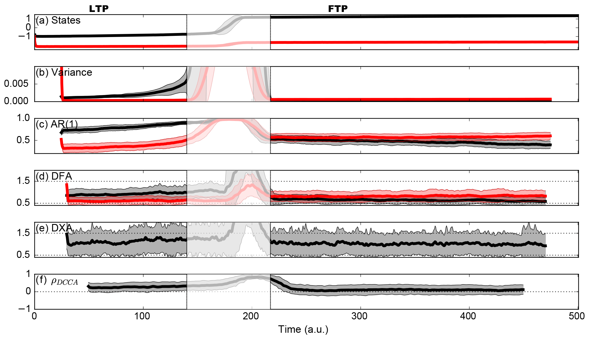
Figure 3 Ensemble (100-member) simulations of a dynamical system undergoing a double-fold cascade (Eq. 13) where both systems undergo a transition, parameter values as in Table 2; (a) states of x (black) and y (red), (b) variance of x (black) and y (red), (c) auto-regressive coefficient at lag 1 of x (black) and y (red), (d) detrended fluctuation analysis scaling exponent of x (black) and y (red), (e) detrended cross-correlation analysis scaling exponent and (f) detrended cross-correlation coefficient by Zebende (2011). White-shaded areas indicate windows containing the actual transitions. The increased variance, AR(1) and the DFA scaling exponent prior to transition in the respective leading system and following system, confirms the predicted increased memory through critical slowing down.
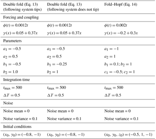
Table 2Parameter values, coupling and initial conditions for the ensemble simulations of the double Fold and fold–Hopf systems as shown in Figs. 3, 4 and 5.
3.3.1 Double-fold cascading tipping
To simulate these events and use statistical indicators, noise has to be included. The system of equations used here is
where in addition to Eq. (3), ζx,ζy are Gaussian white noise terms. We simulate an ensemble of 100 members with the parameter settings and initial conditions as displayed in Table 2. The results of this ensemble are displayed in Fig. 3. Running windows containing the transition are shaded white as these data are misleading when one wants to know what happens before the bifurcation points. We make the distinction between the leading-transitional period (LTP), which is the time series before the tipping point in the leading system, and the following-transitional period (FTP), which is the time series between the first tipping point and the tipping point in the following system. The FTP can be seen as an in-between state that is stable for both systems, although the following system is close to bifurcation, meaning it is rather prone to noise. Therefore, the duration of this state is highly unpredictable. However, as we will see in this section, the FTP does provide information regarding the diagnosis of a potential second transition.
In the LTP, we clearly see the gradual increasing leading system's variance, the AR(1) coefficient and DFA scaling coefficient. These are all evidence of the leading system slowly approaching a bifurcation point, according to the change in the parameter. There is not much evidence of long-range auto-correlations in the time series of the following system, as its variance is low and the DFA scaling exponent remains below 0.5, pointing towards the fact that the detrended fluctuations are statistically white noise. The AR(1) coefficient of the following system does increase just prior to the first tipping, but it also stays small (compared to unity).
The detrended cross-correlation scaling exponent (abbreviated here as DXA) does give >0.5 values, but the range throughout the ensemble members is too large most of the time to see any structural development when approaching the bifurcation point. During the leading system's transition, a strong increase is visible, pointing towards rather strong cross-correlated behaviour during this period (as the following system also shifts its equilibrium a little).
The quantity ρDCCA seems to attain a small positive value (around 0.3) and stays relatively constant throughout the whole time interval. One important aspect of the calculation of ρDCCA, as we found by experimentation, is that the values are very sensitive to the segment size s and the moving window size. The moving window determines the amount of data that is available to find long-range correlations, and the segment size has a strong impact on the accuracy of the fits and on the related segmented fluctuations. Due to the fact that we need a temporal evolution of the statistical indicators in this type of problem, we need moving windows and, thus, encounter a problem. As these indicators (DXA and ρDCCA) have been successfully applied in simpler systems (Podnobik and Stanley, 2008; Zebende, 2011; Zhang et al., 2001; Zhou, 2008), more research on the sensitivity of the indicators with respect to the segment size and moving window size may lead to more robust results.
During the FTP, the variance, AR(1) and DFA of the leading system are strongly reduced. However, the gradual increase of the following system's variance, AR(1) coefficient and DFA scaling coefficient are definitely visible, pointing towards the approach of a bifurcation in the following system. Also notable is the contrast in the DFA of the following system before and after the tipping of x. The DFA of y goes from a white-noise regime (around 0.5) before the tipping of x towards a regime where the detrended fluctuations point to long-range auto-correlations after the tipping of x (1–1.5). This illustrates the relation between the leading system's state and the following system's DFA scaling exponent. The DXA remains relatively high, but overall no structural development is seen in this graph. The quantity ρDCCA exhibits the same behaviour as in the LTP, most likely due to the previously mentioned reasons.
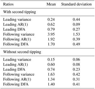
Table 3 Comparison of the ratios of auto-regressive variables prior to and after the first transition, using the ensembles shown in Figs. 3 and 4.
To assess the consequences of the cascading effect on the statistics mentioned, we compare the results with a case where the system (Eq. 13) does not undergo a tipping in the following system (so only one transition remains). The resulting ensemble results are shown in Fig. 4. The most important differences between a regular cascading event and a single tipping event can be found when comparing the variance, AR(1) and DFA scaling coefficient changes between LTP and FTP (or the period after the first transition). During the LTP, the leading system is close to transition and has strong auto-regressive behaviour, whilst the following system is far from its bifurcation point. During the FTP, the following system generally gains memory because it is brought closer to its transition point, and the leading system loses memory because it just arrived at a new state. Therefore, we expect that from the LTP towards the FTP, the variance, AR(1) and DFA will decrease in the leading system, and increase in the following system.
Table 4 Results of Student's t test on the differences between the ratios (in Table 3) of the cases with and without second tipping.
*p-values calculated using the scipy.stats Python package.
To quantify this effect, Table 3 shows the ratios of the different quantities, indicated by Q, during the FTP and LTP phases (), for the cases “with” a second tipping (corresponding to runs shown in Fig. 3) and “without” second tipping (Fig. 4). All ensemble members are included in these values, accounting for a mean and standard deviation of the ratios. As expected, the leading system's auto-regressive metrics decrease in both cases, which is visible in the fact that the mean values of the ratios of the leading system's auto-regressive variables are lower than 1. Furthermore, as expected, the following system's auto-regressive behaviour increases (ratios >1) in both cases; however, it is striking that in the case of a cascading tipping event (with second tipping), the following system's ratios are much higher than those in the case of a single tipping event (without second tipping). To investigate whether the difference in the ratios between single or double tipping is indeed significant, a Student's t test was carried out. The results are shown in Table 4. The high p values for the leading system's ratios indicate no significant difference between single or double tipping, but the low p values for the following system's ratios indicate a significant difference. This shows the potential of using the ratio of auto-regressive variables before and after a transition to assess whether a cascading transition may follow. Further research is needed to quantify this expectation and to assess the sensitivity of these ratios to the system's parameters.
3.3.2 Fold–Hopf cascading tipping
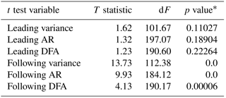
Many statistical indicators have been specifically applied on fold bifurcations, because these transitions show a clear sign of critical slowing down and increased auto-correlation; this is due to their irreversibility and the process of going from one equilibrium towards another. A state approaching a Hopf bifurcation reacts differently to perturbations than a state approaching a saddle-node bifurcation. Therefore, we will consider the fold–Hopf cascade in the light of the previously described statistical indicators. For this, we use the following stochastic dynamical system:
This system is similar to Eq. (4), but white noise is added through the terms ζx, ζy and ζz. We used an ensemble of 100 simulations with the parameter settings and initial conditions as displayed in Table 2. The results of the ensemble are shown in Fig. 5. Here, we do not make the distinction between the LTP and the FTP, because in contrast to the double-fold cascade, the following system undergoes a transition that is easily reversed and the system is either stationary or oscillating. We subtract a running average from the states and calculate the statistics from those series to prevent the oscillation from dominating the signal in the auto-correlation. The following system (red) is quickly drawn towards the equilibrium state , and the leading system (black) is in a steady state. During the time leading up to the bifurcation point, the variance, AR(1) coefficient and DFA of the leading system x gradually increase, as is expected as we force this system towards its bifurcation point. It also seems that the AR(1) of the following system slightly increases during this period.
After the transition of the leading system, the oscillation of the following system immediately starts due to noise. The variance and AR(1) of the following system after the bifurcation are strongly increased with respect to before the bifurcation, despite the removal of the running average to eliminate the oscillation's signal. On average, the DFA scaling exponent of the following system also increases, which relates it to the leading system's state. The DXA sharply increases just prior to the critical transition, although it retains relatively high values throughout the whole time series. The reason behind this might be the low level of noise that is chosen, or other simulation-specific parameters. It could also due to the fact the following system has a high, weakly varying DFA scaling exponent on average, which in turn might affect the height and variability of the cross-correlation. The ρDCCA coefficient remains positive and small, as in the double-fold case. Again, this may have to do with the choice of window and segment sizes.
In this section, we present an application of the concept of cascading tipping (the fold–Hopf case). This application reflects the fact that cascading transitions are not only a purely mathematical concept, but also occur in idealized physical models. Here, we consider cascading tipping in a model that couples the Atlantic meridional overturning circulation (AMOC) and the El Niño–Southern Oscillation (ENSO).
4.1 Background
To demonstrate and quantify the coupling between the AMOC and ENSO, we use output from global climate model simulations. In the ESSENCE project (Ensemble SimulationS of Extreme weather events under Nonlinear Climate changE) several simulations were performed using the ECHAM5/MPI-OM coupled climate model, including so-called “hosing” experiments Sterl et al. (2008), where fresh water is added around Greenland to mimic ice sheet melting.
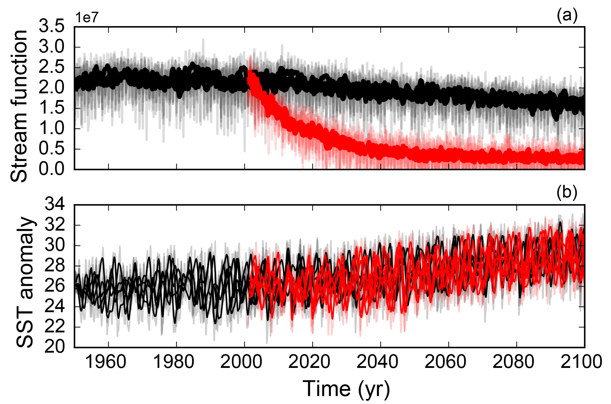
Figure 6(a) Evolution of the five standard SRES-A1b runs (black) and five HOSING-1 runs (red) in terms of the overturning stream function. (b) NINO3.4 of the standard SRES-A1b ensemble (black) and the HOSING-1 ensemble (red). Shaded thin lines indicate monthly means, thick lines indicate the deseasonalised values.
Table 5 NINO3.4 statistics (of deseasonalised data) for the different ensembles. The uncertainty stated is the standard deviation among the five runs within the ensemble. It is visible that in the case of a collapsed overturning, El Niño intensifies more than without a collapsed overturning. Values in bold represent increases in the variability of NINO3.4.
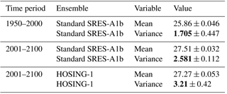
From these climate model simulations we used two ensembles; the first is the “standard” experiment, where greenhouse gases evolve according to observations and from the year 2000 onwards follow the SRES-A1b scenario (experiment name SRES-A1b). The second ensemble is the same as the standard experiment but has additional freshwater input (1 Sv =106 m3 s−1) around Greenland from the end of the year 2000 onwards (experiment name HOSING-1). The HOSING-1 ensemble contains a classical hosing experiment, following the procedure from Jungclaus et al. (2006). Five runs of each ensemble are chosen, specifically runs 041–045 of the HOSING-1 and runs 021–025 of the SRES-A1b ensemble. The temporal resolution used is monthly data between 1950 and 2100. The spatial fields are on a curvilinear grid, with 40 vertical levels in the ocean. We use deseasonalised data because we are interested in interannual variability, not in seasonal variability, as El Niño is associated with these timescales. We use the maximum of the Atlantic meridional overturning stream function at 35∘ N as an AMOC index, and the NINO3.4 index as an ENSO index, which is the average SST over the region 170–120∘ W by 5∘ S–5∘ N.
The results for the evolution of the AMOC and ENSO are shown in Fig. 6. It is clearly visible that the AMOC decreases strongly in the hosing experiments, by approximately 85 %. Table 5 compares statistical properties for the time intervals before and after 2001 (which is the year at which the hosing starts). We use the non-anomaly statistics, as this gives us information about the differences in the mean. We do note that we only use five runs per ensemble, which means that the uncertainty is not statistically robust. We only present it in Table 5 to give the reader an idea of the range of the variables among the different runs.
It is visible from Table 5 that the variability of NINO3.4 increases (bold numbers) if we compare the 1950–2000 and 2001–2100 periods. This increased variability is visible in both the standard and the HOSING-1 runs. However, the variability is much stronger in the HOSING-1 experiment, indicating that the decrease of the AMOC indeed has an amplifying effect on ENSO. The large difference between the standard and hosing runs suggests that the NINO3.4 index changed in the hosing experiment, potentially as a consequence of the decrease of the AMOC. As the first tipping is artificially induced (without any measurable critical slowing down), and the models used here are far more complex than the simple dynamical systems we discussed in previous sections, the question of whether cascading tipping is actually occurring in these runs is beyond the scope of this paper. We only use this data to justify the coupling of AMOC and ENSO.
Several mechanisms have been suggested in the literature regarding the coupling between the AMOC and ENSO. The first mechanism is concerned with oceanic waves. A colder North Atlantic creates density anomalies that induce the southward propagation of oceanic Kelvin waves (along the American coast) across the Equator. In western Africa, this energy radiates as Rossby waves towards the north and south, which induces Kelvin waves to move along the tip of southern Africa into the Indian Ocean, which eventually reach the Pacific. Consequently, the eastern equatorial Pacific thermocline deepens on a decadal timescale. This deepening has a weakening effect on the amplitude of ENSO (Timmermann et al., 2005).
The second mechanism is concerned with the trade winds. Cooling in the northern tropical Atlantic (due to AMOC weakening) induces anticyclonic atmospheric circulation (Xie et al., 2007) that intensifies the northerly trade winds over the northeastern tropical Pacific. This leads to a southward displacement of the Pacific intertropical convergence zone (Zhang and Delworth, 2005) and generates a meridional SST anomaly due to anomalous heat transport and the wind–evaporation–SST feedback in the Pacific. Also, Dong and Sutton (2007) found an atmospheric coupling through Rossby waves sent into the northeast tropical Pacific. This is in line with Dijkstra and Neelin (1995), who argued that part of the contribution to the zonal wind stress, τext, arises from processes outside the tropical Pacific. The result of the wind-stress coupling between the two systems is an intensification of ENSO, and this mechanism is argued to be stronger than the coupling through oceanic waves (Timmermann et al., 2005).
4.2 Models and coupling
To study the possible cascading transition through the wind-stress coupling, we use a conceptual model. For the AMOC, the classical Stommel box model (Stommel, 1961) is used. It consists of a polar (subscript p) and an equatorial box (subscript e), both with a temperature T and salinity S coupled by a density-driven flow rate. The state variables are then defined as and . The time evolution of these variables is as follows (Cessi, 1994):
where the first term in the temperature equation refers to relaxation towards a background temperature, and the second term refers to density-driven meridional transport. Specifically, tr is the surface temperature restoring timescale and θ0 is the equator-to-pole atmospheric temperature difference. Q(Δρ) is the transport function, which is calculated from a diffusion timescale and the meridional density gradient Δρ. In the salinity equation, S0 is a reference salinity, and H is the ocean depth. The parameter Fs is the freshwater flux, which can be used as a bifurcation parameter. The stream function
represents the strength of the AMOC, with γ0>0 a flow constant, ρ0 a reference density and αT, αS the thermal and haline expansion/contraction coefficients.
For the El Niño–Southern Oscillation, we use the conceptual model as proposed in Timmermann et al. (2003). This model has a state vector consisting of the temperature of the western Pacific T1, the temperature of the eastern Pacific T2 and the thermocline depth of the western Pacific h1. The model finds is based on the Zebiak and Cane (1987) ENSO model, with a two-strip and two-box approximation, and a shallow-water model for the upper ocean with a fixed mixed layer depth.
where 1∕α is a typical thermal damping timescale, Tsub is the temperature below the mixed layer, Hm and L are the depths of the mixed layer and the basin width, respectively, w is upwelling velocity and u is atmospheric zonal surface wind linear to wind stress: and . The parameters ϵ and ζ refer to the strength of zonal and vertical advection (bifurcation parameters).
The subsurface temperature Tsub is parameterized as
where h2 is the east equatorial Pacific thermocline depth (calculated as the deviation from a reference depth H), z0 is the depth for which w becomes its characteristic value and h* is the sharpness of the thermocline. The thermocline depths are calculated as follows:
where b is the efficiency of the wind stress τ to drive the thermocline tilt. For further details, we refer to Timmermann et al. (2003). In the Stommel–Timmermann models, we use the standard parameter settings, as given in the references, unless stated otherwise.
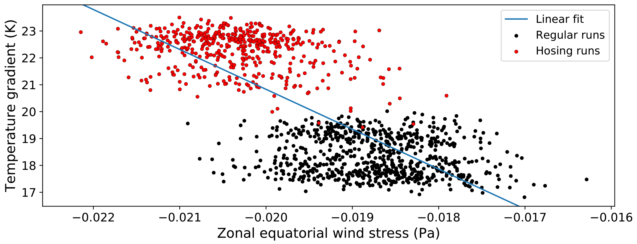
Figure 7 Zonal equatorial wind stress versus the Atlantic temperature gradient. Data from the ESSENCE (Ensemble SimulationS of Extreme weather events under Nonlinear Climate changE) project are used, where the black dots refer to five members of the standard ensemble with SRES-A1b forcing (1950–2100 period ), and the red dots refer to five members of the HOSING-1 ensemble where in 2000 a freshwater perturbation is applied (i.e. 2000–2100 period). A 5-year running mean is applied, yearly averages are shown. The zonal equatorial wind stress is defined here as the average zonal wind stress over the 0–10∘ N latitudinal band. The Atlantic temperature gradient is defined as the difference between the SST in a northern box (50–60∘ N, 50–20∘ W) and a southern box (0–20∘ N, 45–20∘ W). The blue line indicates a linear fit.
We couple the AMOC and ENSO models through the relation between the Atlantic meridional temperature gradient (in the Stommel model) and the Pacific zonal wind stress (in the Timmermann model); the Pacific zonal wind stress mechanism, which is the more important of the two abovementioned mechanisms, is found in the literature, and described in the previous section. Even in a simplified model, the relation between wind stress and meridional temperature gradient is physically justified: thermal wind balance indicates a direct connection between the adjustment of wind stress to changes in the meridional temperature gradient. In the Timmermann model, the zonal wind stress τ is expressed as
with the μ∕β parameters that control the influence of the zonal temperature gradient on the wind stress set to 0.02 Pa⋅ K−1. We add an external wind stress term τext that is dependent on the meridional temperature gradient in the Atlantic ΔT, i.e.
with a negative relation between τext and the Atlantic meridional SST gradient ΔT as we know from the literature described above (a stronger positive ΔT results in stronger easterlies and thus a negative τext). Note that both the Pacific wind stress τ and specifically its external part τext should always be negative. The total wind stress is negative because this area (at low altitude) is strictly dominated by easterly winds, and τext is negative because, through the meridional temperature gradient, it reflects the influence of the zonal mean Hadley cell on the equatorial Pacific. Physically, the Hadley cell only induces negative zonal wind stress in this region.
In the coupling (Eq. 21), we fix β and vary μ as the coupling parameter. For τext we take a linear relation as follows:
where all coefficients are constant over time. The parameters ατ and γτ can be estimated from the ESSENCE data as discussed in Sect. 4.1; τ0 reflects the constant part in the zonal mean wind stress, which we subtract because we are interested in the contribution of changes in the meridional overturning. Using five ESSENCE runs per ensemble for both the standard forcing and hosing-experiment, respectively, ΔT is computed as the absolute difference between the SST in the North Atlantic area (50–60∘ N × 50–20∘ W) and the equatorial Atlantic region (0–20∘ N × 45–20∘ W). For the wind stress τext, the zonally integrated wind stress averaged over the 0–10∘ N region is taken. In Fig. 7, 5-year running means of annual averages are plotted for the hosing simulations (in red) and the standard simulations (in black). Clearly, τext decreases as ΔT increases, meaning that when the AMOC collapses (larger ΔT) the wind stress τext becomes more negative and the external part of the trade winds increases. However, we also note that the spread in the simulation data is large, which can, in part, be attributed to internal variability present in the simulations. The coefficients ατ and γτ were found to be (from a linear fit) −0.000376 Pa ⋅ ∘C−1 and −0.0119 Pa. By looking at the ΔT regime in Fig. 7, τ0 is chosen to be the wind stress at 19 ∘C: Pa. This results in a final quantized expression for the coupling:
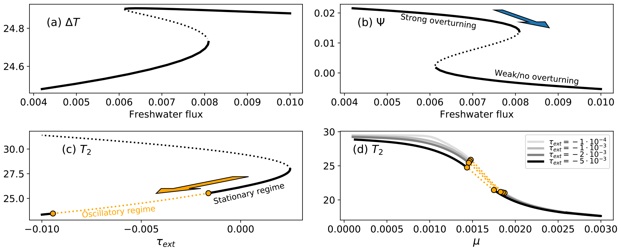
Figure 8Bifurcation diagrams and forward runs of the Stommel (a, b) and Timmermann (c, d) models. The blue arrow indicates the collapse of the overturning circulation, which (negatively) amplifies the external zonal wind stress in the Pacific τext, such that the system enters an oscillatory state. The orange arrow indicates subsequent tipping in the following (ENSO) system. (a) Meridional temperature gradient equilibria versus freshwater flux, and (b) non-dimensional stream function versus freshwater flux. These figures show the multiple states of the overturning. (c) Eastern equatorial Pacific SST versus τext (for μ=0.00145), showing a regime where the system is stationary and a regime where the system is oscillatory; (d) eastern equatorial Pacific SST versus μ for different values of τext. Orange dots indicate Hopf bifurcation points, and orange dotted lines indicate oscillatory regimes. Black and grey solid lines indicate stable equilibria, and black dashed lines indicate unstable equilibria.
4.3 Results
The AMOC model's bifurcation diagrams are shown in Fig. 8a and b, and clearly display a saddle-node structure. For an interval of values of the freshwater flux Fs the system has multiple equilibria, whilst for other values only one equilibrium remains. This means that when we are in the high-Ψ branch and Fs is large enough, the system can make a transition to the low-Ψ branch. This is depicted by the blue arrow in Fig. 8b.
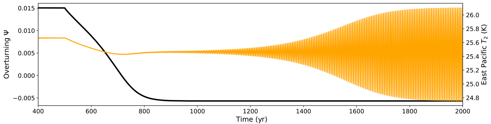
Figure 9Simulation run of the coupled Stommel–Timmermann model for different model configurations, where the collapse of the overturning flow function (black) leads to the crossing of a Hopf bifurcation in the eastern equatorial Pacific SST (orange). Parameter values as in Timmermann et al. (2003), with μ=0.00146.
The bifurcation diagram of the ENSO model with τext as a parameter is shown in Fig. 8c. The bifurcation diagrams become much simpler than in the original Timmermann et al. (2003) model, the reason for this is extensively discussed in Dijkstra and Neelin (1995). Figure 8d shows the influence of μ for the position of the oscillatory regime: on each branch, two Hopf bifurcations can be found and the μ value of the first Hopf bifurcation decreases with more negative τext. This indicates that a Hopf bifurcation can be crossed if τext is decreased, while μ is kept constant. In other words, for the right value of μ, the eastern Pacific SST starts oscillating (El Niño “intensifies”) when the easterly external wind is increased. For the coupled model, we use μ=0.00146.
Using τext to couple the AMOC and ENSO models, we performed simulations with Δt=0.1 days and the Runge–Kutta fourth-order integration method. To initiate the collapse of the overturning, a freshwater forcing Fs is applied in the form of a step function:
Using the coupling of Eq. (23), we attain the results shown in Fig. 9. The exact quantification of the coupling partly modulates which effect the collapse of the AMOC has on ENSO. For the chosen coupling, the collapse of the overturning leads to the crossing of the first Hopf bifurcation point in the following system, and an oscillation starts growing. As is visible in Fig. 6, the relation between ΔT and τ has quite some spread, which implies a large uncertainty in the values of ατ and γτ. We would like to stress that the regime in which the Hopf bifurcation is crossed is dependent on multiple variables, such as these coupling parameters. Running the forward integration of the coupled model for values between and , uncovers the fact that (ceteris paribus), for higher (lower) values of ατ, the oscillation indeed becomes weaker (stronger), finally resulting in a disappearance of the oscillation at at a time step of 0.25 days.
Despite the parameter sensitivity, this is a typical illustration of the fold–Hopf cascading behaviour discussed in earlier sections. This re-enforces the possibility that cascading transitions are possible in real physical systems.
In this paper, we introduced the concept of cascading tipping, which can occur when a transition in a leading system alters background conditions for a following system that then undergoes a transition. We presented a mathematical framework around this concept, using generic bifurcations (saddle-node and Hopf) in both leading and following systems. Four types of deterministic dynamical systems with the possibility for cascading events were formulated, including the double-fold cascade, the fold–Hopf cascade, the Hopf–fold cascade and the double-Hopf cascade. In all cases we assumed a linear coupling between the following and leading system. The double-fold coupled system has previously been considered in another context (Brummitt et al., 2015), where it was also noted that not all subsystems undergo tipping (“hopping”) in systems with more than two coupled fold cascades. Moreover, stochastically coupled multi-stable systems have been considered in networks, where different types of domino effects can occur depending on the synchrony of the transition in the different network nodes (Ashwin et al., 2017; Creaser et al., 2018). Here we only consider two coupled systems, but allow different types of bifurcations, and the systems are physically coupled in a directional way.
We discussed statistical indicators and analysis tools for cascading tipping points. Indicators for cascading tipping points are found in detrended cross-correlation analysis (DCCA) and a special case of extrapolation using the DFA of the following system. These tools were applied in simulations involving both the double-fold and fold–Hopf cascades. The increased variance, AR(1) and DFA scaling exponent are clearly found in each case of single tipping. The cross-correlation indicators (DCCA and ρDCCA) did not evolve much throughout the time series, which indicates their insensitivity with respect to the proximity to single tipping points. Several limitations on the use of these variables have been mentioned. However, it seems that these metrics are highly sensitive to window and segment sizes, which means that their potential as early warnings of cascading transition events is inconclusive. The ratios of auto-regressive metrics before and after the first transition seem to be a stronger warning of cascading transitions. More research is needed to exactly quantify these metrics.
The concept of cascading tipping was applied to study the behaviour of a model describing a link between the Atlantic meridional overturning circulation (MOC) and ENSO. We modelled this using a coupling between the Stommel (1961) model and the Timmermann et al. (2003) ENSO model by a meridional temperature gradient-dependent term in the external wind stress of the ENSO model. Through analysis of the bifurcation diagrams and simulations, a cascading tipping event is indeed possible within this model in the form of the fold–Hopf cascade. Obviously, both models are highly idealized and more detailed models of both AMOC and ENSO are needed to demonstrate the occurrence of such a cascading transition in the climate system.
A potential example of a double-fold cascade, which was not further treated here, could be the impact of a bistable MOC on the (bistable) land ice formation on the Antarctic continent. In this case the coupling exists through the atmospheric CO2 concentration, which depends on mixing and circulation in the ocean while strongly determining the existence of an ice sheet DeConto and Pollard (2003). During the Eocene–Oligocene transition, where a large ice sheet grew on Antarctica, a two-step signal is observed in the deep-sea δ18O ratio, suggesting two abrupt transitions. Using a box model by Gildor and Tziperman (2000), Tigchelaar et al. (2011) showed that a two-step signal can be produced by (first) a MOC transition which changes the CO2 concentration meaning that a transition occurs in the land-ice model. Although from a physical perspective, this is a potential example of a cascading transition, we make no claim about whether such a transition likely occurred at the Eocene–Oligocene transition. Here, more detailed models are also needed and transition are expected to be more complicated (Tantet et al., 2018).
These two applications reflect the relevance of this paper. There are likely many cases in which these cascading events occur in climate and therefore highlight the importance of the topic. Future research will point out whether these events are likely to happen in the future climate and whether these effects also occur in fields other than climate science. Of course, this paper covers the very basics of deterministic cascading events. However, one can imagine a wide range of phenomena if more complicated transitions between attractors are considered and when noise is included. For example, when a leading chaotic system is coupled to a deterministic following system with a saddle-node bifurcation structure, a slight change in the chaotic attractor may change the background conditions for the following system such that it undergoes a transition. An application here may be the effect of a mid-latitude atmospheric jet on the Atlantic MOC. We hope that this paper will stimulate more research on the various types of cascading tipping and also on the development of well-suited indicators and early warnings of such events.
Models, analysis scripts and outputs are available on request from the corresponding author.
All authors developed the research idea, MMD carried out the computations and performed the analysis. All authors discussed the results and contributed to writing the paper.
The authors declare that they have no conflict of interest.
Anna S. von der Heydt and Henk A. Dijkstra acknowledge support from the
Netherlands Earth System Science Centre (NESSC), financially supported by the
Ministry of Education, Culture and Science (OCW), grant no. 024.002.001.
Anna S. von der Heydt thanks Peter Ashwin for discussions related to this
work. She is also grateful to the University of Exeter and the EPSRC funded
Past Earth Network (grant no. EP/M008363/1) for funding an extended visit to
the University of Exeter during the Summer of 2017.
Edited by: Valerio Lucarini
Reviewed by:
Alexis Tantet and one anonymous referee
Aleina, F. C., Baudena, M., D'Andrea, F., and Provenzale, A.: Multiple equilibria on planet Dune: Climate-vegetation dynamics on a sandy planet, Tellus B, 65, 17662, https://doi.org/10.3402/tellusb.v65i0.17662, 2013. a
Ashwin, P., Wieczorek, S., Vitolo, R., and Cox, P.: Tipping points in open systems: Bifurcation, noise-induced and rate-dependent examples in the climate system, Philos. T. Roy. Soc. A, 370, 1166–1184, https://doi.org/10.1098/rsta.2011.0306, 2012. a
Ashwin, P., Creaser, J., and Tsaneva-Atanasova, K.: Fast and slow domino effects in transient network dynamics, Phys. Rev. E, 96, 052309, https://doi.org/10.1103/PhysRevE.96.052309, 2017. a
Barriopedro, D., García-Herrera, R., Lupo, A. R., and Hernández, E.: A Climatology of Northern Hemisphere Blocking, J. Climate, 19, 1042–1063, https://doi.org/10.1175/JCLI3678.1, 2006. a
Bathiany, S., van der Bolt, B., Williamson, M. S., Lenton, T. M., Scheffer, M., van Nes, E. H., and Notz, D.: Statistical indicators of Arctic sea-ice stability – prospects and limitations, The Cryosphere, 10, 1631–1645, https://doi.org/10.5194/tc-10-1631-2016, 2016. a, b
Brummitt, C. D., Barnett, G., and D'Souza, R. M.: Coupled catastrophes: sudden shifts cascade and hop among interdependent systems, J. R. Soc. Interface, 12, https://doi.org/10.1098/rsif.2015.0712, 2015. a
Cessi, P.: A simple box model of stochastically forced thermohaline flow, J. Phys. Oceanogr., 24, 1911–1920, 1994. a
Creaser, J., Tsaneva-Atanasova, K., and Ashwin, P.: Sequential noise-induced escapes for oscillatory network dynamics, SIAM J. Appl. Dyn. Syst., 17, 500–525, https://doi.org/10.1137/17M1126412, 2018. a
Dakos, V., Scheffer, M., van Nes, E. H., Brovkin, V., Petoukhov, V., and Held, H.: Slowing down as an early warning signal for abrupt climate change, P. Natl. Acad. Sci. USA, 105, 14308–14312, https://doi.org/10.1073/pnas.0802430105, 2008. a
DeConto, R. M. and Pollard, D.: Rapid Cenozoic glaciation of Antarctica induced by declining atmopsheric CO2, Nature, 421, 245–249, 2003. a, b
Dijkstra, H. A. and Neelin, D.: Ocean-Atmosphere Interaction and the Tropical Climatology. Part II: Why the Pacific Cold Tongue is in the East, J. Climate, 8, 1343–1359, 1995. a, b
Dong, B. and Sutton, R.: Enhancement of ENSO Variability by a Weakened Atlantic Thermohaline Circulation in a Coupled GCM, J. Climate, 20, 4920–4939, https://doi.org/10.1175/JCLI4284.1, 2007. a, b
Elsworth, G., Galbraith, E., Halverson, G., and Yang, S.: Enhanced weathering and CO2 drawdown caused by latest Eocene strengthening of the Atlantic meridional overturning circulation, Nat. Geosci., 10, 213–216, https://doi.org/10.1038/ngeo2888, 2017. a
Gasson, E., Lunt, D. J., DeConto, R., Goldner, A., Heinemann, M., Huber, M., LeGrande, A. N., Pollard, D., Sagoo, N., Siddall, M., Winguth, A., and Valdes, P. J.: Uncertainties in the modelled CO2 threshold for Antarctic glaciation, Clim. Past, 10, 451–466, https://doi.org/10.5194/cp-10-451-2014, 2014. a
Gildor, H. and Tziperman, E.: Sea ice as the glacial cycles' Climate switch: role of seasonal and orbital forcing, Paleoceanography, 15, 605–615, https://doi.org/10.1029/1999PA000461, 2000. a
Held, H. and Kleinen, T.: Detection of climate system bifurcations by degenerate fingerprinting, Geophys. Res. Lett., 31, l23207, https://doi.org/10.1029/2004GL020972, 2004. a, b, c, d
Hirota, M., Holmgren, M., Van Nes, E. H., and Scheffer, M.: Global Resilience of Tropical Forest and Savanna to Critical Transitions, Science, 334, 232–235, https://doi.org/10.1126/science.1210657, 2011. a
Jungclaus, J. H., Haak, H., Esch, M., Roeckner, E., and Marotzke, J.: Will Greenland melting halt the thermohaline circulation?, Geophys. Res. Lett., 33, l17708, https://doi.org/10.1029/2006GL026815, 2006. a
Kriegler, E., Hall, J. W., Held, H., Dawson, R., and Schellnhuber, H.: Imprecise Probability Assessment of Tipping Points in the Climate System, P. Natl. Acad. Sci. USA, 106, 5041–5046, 2009. a
Kuehn, C.: A mathematical framework for critical transitions: Bifurcations, fast-slow systems and stochastic dynamics, Physica D, 240, 1020–1035, https://doi.org/10.1016/j.physd.2011.02.012, 2011. a, b, c
Kutzbach, J., Bonan, G., Foley, J., and Harrison, S.: Vegetation and soil feedbacks on the response of the African monsoon to orbital forcing in the early to middle Holocene, Nature, 384, 623–626, https://doi.org/10.1038/384623a0, 1996. a
Lenton, T. M.: Early Warning of Climate Tipping Points, Nat. Clim. Change, 1, 201–209, 2011. a
Lenton, T. M. and Williams, H. T.: On the origin of planetary-scale tipping points, Trends Ecol. Evol., 28, 380–382, https://doi.org/10.1016/j.tree.2013.06.001, 2013. a, b
Lenton, T. M., Held, H., Kriegler, E., Hall, J. W., Lucht, W., Rahmstorf, S., and Schellnhuber, H. J.: Tipping elements in the Earth's climate system, P. Natl. Acad. Sci. USA, 105, 1786–1793, https://doi.org/10.1073/pnas.0705414105, 2008. a
Livina, V. and Lenton, T.: A modified method for detecting incipient bifurcations in a dynamical system, Geophys. Res. Lett., 34, l03712, https://doi.org/10.1029/2006GL028672, 2007. a, b, c, d, e
Pearson, P., Foster, G., and Wade, B.: Atmospheric carbon dioxide through the Eocene–Oligocene climate transition, Nature, 461, 1110–1113, 2009. a
Peng, C.-K., Buldyrev, S. V., Havlin, S., Simons, M., Stanley, H. E., and Goldberger, A. L.: Mosaic organization of DNA nucleotides, Phys. Rev. E, 49, 1685–1689, https://doi.org/10.1103/PhysRevE.49.1685, 1994. a, b, c
Podnobik, B. and Stanley, H.: Detrended Cross-Correlation Analysis: A New Method for Analyzing Two Non-stationary Time Series, Phys. Rev. Lett., 100, 084102, https://doi.org/10.1103/PhysRevLett.100.084102, 2008. a, b, c, d
Scheffer, M., Bascompte, J., Brock, W., Brovkin, V., Carpenter, S., Dakos, V., Held, H., van Nes, E., Rietkerk, M., and Sugihara, G.: Early-warning signals for critical transitions, Nature, 461, 53–59, https://doi.org/10.1038/nature08227, 2009. a, b, c
Sterl, A., Severijns, C., Dijkstra, H. A., Hazeleger, W., van Oldenborgh, G. J., van den Broeke, M., Burgers, G., van den Hurk, B., van Leeuwen, P. J., and van Velthoven, P.: When can we expect extremely high surface temperatures?, Geophys. Res. Lett., 35, L14703, https://doi.org/10.1029/2008GL034071, 2008. a
Stommel, H.: Thermohaline Convection with Two Stable Regimes of Flow, Tellus A, 13, 224–230, https://doi.org/10.1111/j.2153-3490.1961.tb00079.x, 1961. a, b, c
Tantet, A., Lucarini, V., and Dijkstra, H. A.: Resonances in a Chaotic Attractor Crisis of the Lorenz Flow, J. Stat. Phys., 170, 584–616, https://doi.org/10.1007/s10955-017-1938-0, 2018. a, b
Thompson, J. and Stewart, H.: Nonlinear Dynamics and Chaos, Wiley, available at: https://books.google.nl/books?id=vQvu-5VPkmcC (last access: 2 November 2018), 2002. a
Thompson, J. M. T. and Sieber, J.: Predicting Climate Tipping as a noisy bifurcation: a review, Int. J. Bifurcat. Chaos, 21, 399–423, https://doi.org/10.1142/S0218127411028519, 2011. a, b, c
Tigchelaar, M., von der Heydt, A. S., and Dijkstra, H. A.: A new mechanism for the two-step δ18O signal at the Eocene-Oligocene boundary, Clim. Past, 7, 235–247, https://doi.org/10.5194/cp-7-235-2011, 2011. a, b
Timmermann, A., Jin, F., and Abshagen, J.: A Nonlinear Theory for El Niño Bursting, J. Atmos. Sci., 60, 152–165, https://doi.org/10.1175/1520-0469(2003)060<0152:ANTFEN>2.0.CO;2, 2003. a, b, c, d, e
Timmermann, A., An, S.-I., Krebs, U., and Goosse, H.: ENSO Suppression due to Weakening of the North Atlantic Thermohaline Circulation, J. Climate, 18, 3122–3139, https://doi.org/10.1175/JCLI3495.1, 2005. a, b, c
Timmermann, A., Okumura, Y., An, S.-I., Clement, A., Dong, B., Guilyardi, E., Hu, A., Jungclaus, J. H., Renold, M., Stocker, T. F., Stouffer, R. J., Sutton, R., Xie, S.-P., and Yin, J.: The Influence of a Weakening of the Atlantic Meridional Overturning Circulation on ENSO, J. Climate, 20, 4899–4919, https://doi.org/10.1175/JCLI4283.1, 2007. a
Xie, S.-P., Miyama, T., Wang, Y., Xu, H., de Szoeke, S. P., Small, R. J. O., Richards, K. J., Mochizuki, T., and Awaji, T.: A Regional Ocean–Atmosphere Model for Eastern Pacific Climate: Toward Reducing Tropical Biases, J. Climate, 20, 1504–1522, https://doi.org/10.1175/JCLI4080.1, 2007. a
Yuan, N., Zuntau, F., Zhang, H., Piao, L., Xoplaki, E., and Luterbacher, J.: Detrended Partial-Cross-Correlation Analysis: A New Method for Analyzing Correlations in Complex System, Sci. Rep., 5, 8143, https://doi.org/10.1038/srep08143, 2015. a
Zebende, G.: {DCCA} cross-correlation coefficient: Quantifying level of cross-correlation, Physica A, 390, 614–618, https://doi.org/10.1016/j.physa.2010.10.022, 2011. a, b, c, d
Zebiak, S. E. and Cane, M. A.: A Model El Niño–Southern Oscillation, Mon. Weather Rev., 115, 2262–2278, https://doi.org/10.1175/1520-0493(1987)115<2262:AMENO>2.0.CO;2, 1987. a
Zhang, D., Lee, T. N., Johns, W. E., Liu, C.-T., and Zantopp, R.: The Kuroshio East of Taiwan: Modes of Variability and Relationship to Interior Ocean Mesoscale Eddies, J. Phys. Oceanogr., 31, 1054–1074, https://doi.org/10.1175/1520-0485(2001)031<1054:TKEOTM>2.0.CO;2, 2001. a, b, c
Zhang, R. and Delworth, T. L.: Simulated Tropical Response to a Substantial Weakening of the Atlantic Thermohaline Circulation, J. Climate, 18, 1853–1860, https://doi.org/10.1175/JCLI3460.1, 2005. a
Zhou, W.: Multifractal detrended cross-correlation analysis for two nonstationary signals, Phys. Rev., 77, 066211, https://doi.org/10.1103/PhysRevE.77.066211, 2008. a, b, c