the Creative Commons Attribution 4.0 License.
the Creative Commons Attribution 4.0 License.
 | 08 Apr 2020
Statistical estimation of global surface temperature response to forcing under the assumption of temporal scaling
Eirik Myrvoll-Nilsen
Sigrunn Holbek Sørbye
Hege-Beate Fredriksen
Håvard Rue
Martin Rypdal
Reliable quantification of the global mean surface temperature (GMST) response to radiative forcing is essential for assessing the risk of dangerous anthropogenic climate change. We present the statistical foundations for an observation-based approach using a stochastic linear response model that is consistent with the long-range temporal dependence observed in global temperature variability. We have incorporated the model in a latent Gaussian modeling framework, which allows for the use of integrated nested Laplace approximations (INLAs) to perform full Bayesian analysis. As examples of applications, we estimate the GMST response to forcing from historical data and compute temperature trajectories under the Representative Concentration Pathways (RCPs) for future greenhouse gas forcing. For historic runs in the Model Intercomparison Project Phase 5 (CMIP5) ensemble, we
estimate response functions and demonstrate that one can infer the transient climate response (TCR) from the instrumental temperature record. We illustrate the effect of long-range dependence by comparing the results with those obtained from one-box and two-box energy balance models. The software developed to perform the given analyses is publicly available as the R package INLA.climate.


Despite decades of research and development regarding global circulation models (GCMs) and Earth system models (ESMs), the discrepancies between models remain substantial, even as we describe physical processes with increasing accuracy and resolution. Part of the model spread is associated with a lack of understanding of the shortwave cloud feedback (Qu et al., 2018). However, there are several other modeling choices and compromises that contribute to the uncertainty (Flato, 2011). As a consequence, several studies have focused on constraining model results on climate sensitivity on observational data; see, e.g., the work of Annan and Hargreaves (2006) or the more recent studies of Cox et al. (2018) and Rypdal et al. (2018b, a). These studies focus on the equilibrium climate sensitivity (ECS) as an essential metric of the climate response, as have numerous paleoclimate studies (Hansen et al., 2013; von der Heydt and Ashwin, 2017; Köhler et al., 2017).
A simpler approach is to adopt a linear approximation and to apply statistical methods to extract information on the climate response from data on global surface temperature and radiative forcing in the instrumental era. Under the assumption of a linear and stationary response, the global surface temperature anomaly ΔT can be expressed as a filtering of the global radiative forcing F, mathematically expressed as
where σdB(t) represents a white-noise forcing that gives rise to internal climate variability, and G is the response function, or Green's function, characterizing the relation between forcing and the temperature anomaly. A model of this form can arise from the simplest energy balance model, i.e., the equations
and ΔQ=CΔT, where ΔQ is the change in the system's heat content corresponding to a temperature change ΔT, and C is heat capacity (Rypdal, 2012). If a white-noise forcing term is included on the right-hand side of Eq. (2) it becomes a stochastic differential equation with a stationary solution to the form of Eq. (1), with and . The process has a natural decomposition into the response to the known forcing,
and a stochastic term,
which for this particular model is an Ornstein–Uhlenbeck process. Rypdal and Rypdal (2014) show how the parameters of the two terms can be estimated simultaneously from time series of forcing and the GMST using the maximum likelihood (ML) method. They also demonstrate that the resulting process is inconsistent with observations. The stochastic term X(t) does not exhibit the strong positive decadal-scale serial correlations that are observed in the GMST in the instrumental era, and the model's response to reconstructed forcing for the last millennium does not show sufficient low-frequency variability compared to Northern Hemisphere temperature reconstructions.
The inconsistency of the simple energy balance model is due to the slow climate response associated with the energy exchange with the deep ocean. One can easily incorporate this effect within the framework of Eq. (1) by generalizing the zero-dimensional (one-box) model to a two-box model that includes a layer representing the deep ocean (Geoffroy et al., 2013; Held et al., 2010; Caldeira and Myhrvold, 2013) or the more general m-box model discussed by Fredriksen and Rypdal (2017).
The generalization from the zero-dimensional (one-box) energy balance model to the two-box model, or the m-box models, means that the number of free parameters increases. Concerning statistical inference, this could be problematic due to potential over-fitting. Mathematically, the generalization of Eq. (2) is of the form
where the diagonal elements of C are the heat capacities of each box, and the matrix K contains coefficients describing heat exchange between boxes and the feedback parameter λ.
The system in Eq. (5) is solved by bringing the matrix C−1K to diagonal form, and the surface temperature anomaly can be written as in Eq. (1), where G(t) is the weighted sum of m exponential functions (Fredriksen and Rypdal, 2017):
The characteristic timescales are defined from the eigenvalues μk of C−1K, and wk denotes the weight of the kth exponential function.
On the other hand, global temperature variability exhibits a scaling symmetry. For instance, both the forced and the unforced global temperature variability have power spectral densities (PSDs) that are approximate power laws,
for frequencies corresponding to timescales ranging from months to centuries (Rypdal and Rypdal, 2016; Rybski et al., 2006; Lovejoy and Schertzer, 2013; Huybers and Curry, 2005; Franzke, 2010; Fredriksen and Rypdal, 2016). The global temperature fluctuations are consistent with a fractional Gaussian noise (fGn), which can formally be defined by the integral analogous to Eq. (4), but with the exponential response function replaced with a scale-invariant response function:
Here, γ is a scale parameter with the dimension of time, and ξ is a variable needed in order for G(t) to have the correct physical dimensions. The scaling exponent β (defined from the PSD in Eq. 7) relates to the so-called Hurst exponent of the fGn via the formula . Based on this Rypdal and Rypdal (2014) proposed a fractional linear response model in the form of Eq. (1), in which the parsimonious expression in Eq. (8) replaces the linear combination of exponential functions in Eq. (6). The cost of the reduction in model complexity is that the fractional linear response model does not have a well-defined ECS, and in general, we cannot write the model as a system of differential equations as in Eq. (5). But on timescales up to approximately 103 years, the model provides an accurate description of both forced and unforced surface temperature fluctuations (Rypdal and Rypdal, 2014; Rypdal et al., 2015), and the millennial-scale climate sensitivity in the estimated fractional linear response model correlates strongly with ECS over the ensemble of models in the Coupled Model Intercomparison Project Phase 5 (CMIP5) (Rypdal et al., 2018a).
Temporal-scale invariance in global temperature fluctuations is an empirical observation and we cannot deduce the parameters in the fractional linear response model from physical principles. This paper presents a statistical methodology that makes it possible to fit the model to observational data and estimate all model parameters. Parameter estimation is done within a Bayesian framework by making use of the methodology of integrated nested Laplace approximation (INLA) for latent Gaussian models introduced in Rue et al. (2009). Barboza et al. (2019) use this framework to investigate model formulations and forcing components in paleoclimate reconstructions.
The INLA methodology and inference for our statistical model, assuming the scale-invariant response function in Eq. (8), are described further in Sect. 2. This section explains how to compute the marginal posterior distributions of the model parameters. As the model has a nonstandard form, this includes certain modifications of the INLA methodology to ensure computational efficiency. We discuss applications in Sect. 3.
In Sect. 3.1 we fit the model to the temperature and forcing dataset generated by the GISS-E2-R (Schmidt et al., 2014) ESM. Here we show how to extract the GMST response to the known forcing using a Monte Carlo sampling approach. In Sect. 3.2, the model is used for temperature forecasting wherein the Representative Concentration Pathway (RCP) trajectories describe the future CO2 forcing. Section 3.3 describes how the transient climate response (TCR) can be estimated using our model. We obtain estimates for 19 temperature series and their associated adjusted forcing series.
We compare the resulting estimates of TCRs with the TCRs obtained directly from the respective ESMs and with TCR estimates from the historical HadCRUT4 temperature dataset using different forcing data. The applications are incorporated in the R package INLA.climate. This package also includes the option of using the exponential response functions as defined by Eqs. (3) and (4) for the one-box model and Eq. (6) for m-box models. A discussion and final conclusions are given in Sect. 4.
Rypdal and Rypdal (2014) use an ML estimator to estimate the model parameters from the observational yearly time series of of GMST and the corresponding vector of radiative forcing . Here, we estimate parameters by adopting a Bayesian framework, making use of the INLA methodology (Rue et al., 2009, 2017). This approach implies that parameters are treated as stochastic variables and assigned prior distributions. The information given by the priors is then combined with the likelihood of the observations and updated to give posterior distributions using Bayes' theorem.
In a discrete-time model, we assume that ΔTt has a Gaussian distribution with a random mean expressed by the linear predictor
where , while F0 denotes a shift parameter that gives the initial forcing value. Gts denotes a discretely indexed element of the function,
Further, the vector denotes a zero-mean fGn process, implying that the covariance between εt and εs is
where σε=σσf. In vector notation, the predictor is then given by
where
The covariance matrix of the predictor is with the elements in Eq. (11). Notice that the matrix G(H) is lower triangular with elements given by Eq. (10). The given formulation implies that the vector μ represents the GMST response to the known forcing F, while ε is the GMST response to the random forcing, i.e., the unforced climate variability.
The statistical regression formulation in Eq. (9) has a hierarchical structure in which the expected temperature anomalies are modeled in terms of the random predictor η with elements specified by Eq. (9). The predictor depends on additional model parameters . This setup implies that we need to assign priors to both the predictor and the model parameters. By assigning a Gaussian prior to η, the resulting model becomes a latent Gaussian model, which can be analyzed using the INLA methodology. In general, this class of models introduces a latent Gaussian field x, which contains all the random components of a linear predictor, including the predictor itself. In our case, the latent field is equal to the linear predictor, However, inference for this model is not straightforward as the model parameter H appears in both of the terms μ and ε. We choose to circumvent this problem by considering the sum μ+ε to be a single model component, i.e., as a fractional Gaussian noise process with mean vector μ and covariance matrix Σ. The dependence between two components implies that we will not get separate posterior estimates for μ and ε directly.
Using p(⋅) as a generic notation for probability density functions, we can summarize the three-stage hierarchical structure of latent Gaussian models, including distributional assumptions, as follows.
-
The first stage specifies the likelihood of the model. The observed temperature anomaly ΔTt is assigned a Gaussian distribution with negligible fixed variance and mean ηt. The observations are assumed to be conditionally independent given the latent field x and parameters θ, i.e.,
-
The second stage specifies the prior distribution for the latent field. Given the parameters θ, the latent field x is assigned a Gaussian prior distribution with mean vector and precision matrix, , defined as the inverse covariance matrix, i.e.,
-
The third stage specifies independent priors for the parameters:
The shift parameter F0 is assigned a zero-mean Gaussian prior, while the other parameters are assigned penalized complexity (PC) priors (Simpson et al., 2017). The class of PC priors represents a recently developed framework to compute priors based on specific principles, including support for Occam's razor. The PC prior of the two scaling parameters σf and σϵ can be computed to equal the exponential distribution, while the PC prior of H is computed numerically (Sørbye and Rue, 2018).
The joint posterior for all components of the latent field and all of the model parameters is then summarized by
Our main objective is to estimate the marginal posterior distribution for all components of the latent field
and the marginal posteriors for all the model parameters
Here, the notation θ−j is used to denote the vector θ excluding the jth parameter. The posterior distributions provide a complete description of the latent field components and the parameters in our model. From the marginals in Eqs. (14)–(15) we can extract summary statistics such as the mean, variance, quantiles, and credible intervals.
Traditionally, marginal posterior distributions have been approximated using Markov chain Monte Carlo methods (Robert and Casella, 1999). Such methods are simulation-based and can potentially be very time-consuming for hierarchical models. The INLA methodology represents a computationally superior, but still accurate, alternative and is available using the R package R-INLA. This package can be downloaded for free at http://www.r-inla.org (last access: 10 December 2019). INLA provides a deterministic approach by approximating the posterior distributions in Eqs. (14)–(15) using numerical optimization techniques, interpolations, and numerical integration.
Among other features, this includes the use of the Laplace approximation (Tierney and Kadane, 1986), which is an old technique to compute high-dimensional integrals.
Specifically, the joint posterior distribution for the model parameters in Eq. (15) is approximated by employing a Laplace approximation evaluated at the mode x∗(θ):
where is a Gaussian approximation of
This approximation is usually very accurate as we know that p(x|θ) is already Gaussian. The marginal for each model parameter is then obtained by assuming a normal distribution modified to allow for skewness,
The scaling parameters σj+ and σj− are found using the approximate joint posterior distribution of Eq. (16); see Martins et al. (2013) for details. To compute Eq. (14), the Laplace approximation in Eq. (16) is combined with a simplified and computationally faster version of the Laplace approximation of . Finally, the integrand of Eq. (14) is evaluated for values of θ in a grid efficiently covering the parameter space for θ; see Rue et al. (2009, 2017) for details.
A key assumption for the numerical approximations to be computationally efficient is that the latent Gaussian field x has Markov properties; i.e., x needs to be a Gaussian Markov random field having a sparse precision matrix Q (Rue and Held, 2005). This is not the case for fGn as the long-range dependency structure of this process gives a dense precision matrix. We resolve this problem by approximating ε as a weighted sum of m independent first-order autoregressive (AR(1)) processes, i.e.,
To capture the correlation structure between and each of the AR(1) processes , the latent field must be extended to also include the underlying AR(1) processes, i.e., . The weights and the first-lag autocorrelation coefficients of the AR(1) processes are selected such that the resulting autocorrelation function of best approximates that of fGn. In addition to ensuring computational efficiency, this approximation also proves to be remarkably accurate. For further details about this approximation, see Sørbye et al. (2019), who also provide a discussion from a statistical perspective. For a physical interpretation of this approximation we refer to Fredriksen and Rypdal (2017).
Currently, there are no built-in model components in R-INLA that suit our specifications. This means that we have to construct one manually using rgeneric, a modeling tool that allows generic model components to be defined for INLA.
To make this accessible to applied scientists we have developed an R package called INLA.climate, which includes functions that take care of the technical part of the fitting procedure and presents important information and summary statistics in a readable format. This package contains a versatile and user-friendly interface to fit the model in Eq. (9) and includes functions to replicate all results presented in this paper. The package is available at the GitHub repository at https://github.com/eirikmn/INLA.climate (last access: 11 February 2020).
A detailed description of the package and its features is available in its accompanying documentation.
3.1 Estimating the forced temperature response
As explained in Sect. 2, our model formulation implies that the sum μ+ε is viewed as one model component. Consequently, INLA will give an estimate for the posterior distribution of the sum, and not the marginal posterior distributions for each of the terms μ and ε.

Figure 1The marginal posterior distributions of the parameters obtained using INLA.climate to fit our model to the GISS-E2-R temperature and forcing dataset. The vertical lines show the mean and 95 % credible intervals.
In this example, we illustrate how we can approximate the marginal posterior distribution for the temperature response attributed to the known forcing, p(μi|ΔT) by combining INLA with Monte Carlo sampling. We first fit our model to the GISS-E2-R temperature and the corresponding forcing data using INLA. This gives the estimated marginal posterior distributions for each of the model parameters , as shown in Fig. 1.
Next, we use the inla.hyperpar.sample function from the R-INLA package to draw 100 000 samples from the approximate joint posterior distribution of H,σf, and F0. For each of these samples, we compute μ according to Eq. (13). The resulting samples give approximate marginal posterior distributions for each μi, which can then be used to calculate summary statistics.
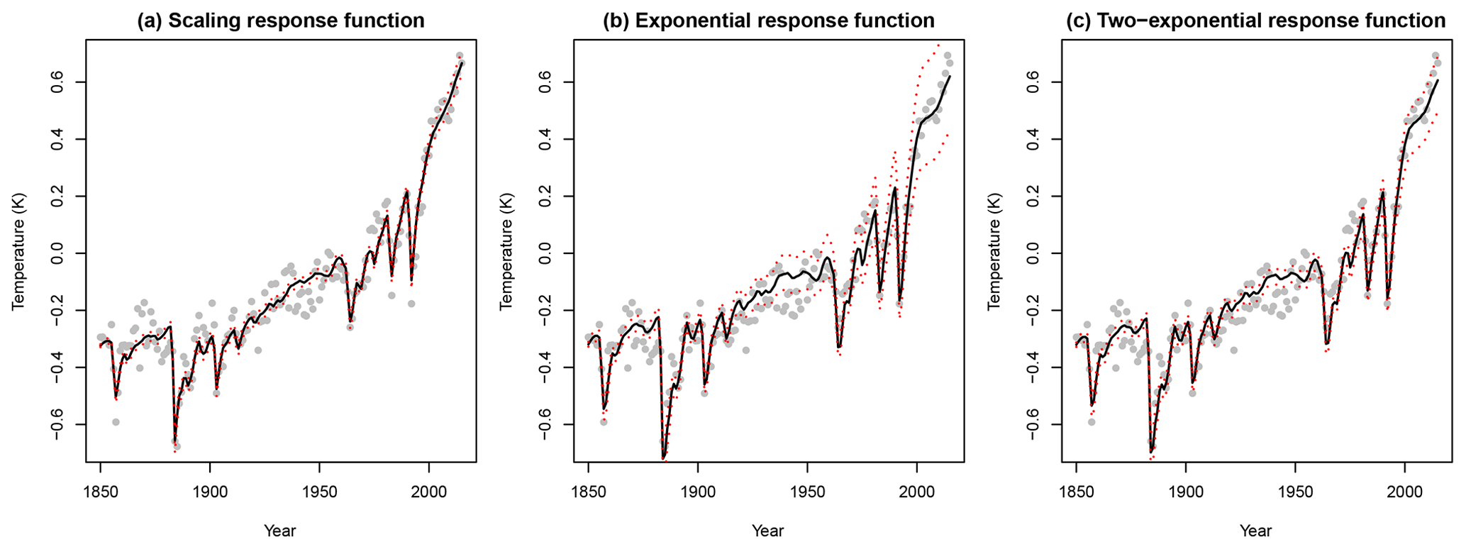
Figure 2The marginal posterior mean and 95 % credible intervals of the temperature response to known forcing μ obtained by 100 000 Monte Carlo simulations compared to GISS-E2-R temperature data. Panel (a) shows the results under the scale-invariant assumption, panel (b) shows the results using a single-exponential response, and panel (c) shows the results using a mixture of two-exponential response functions.
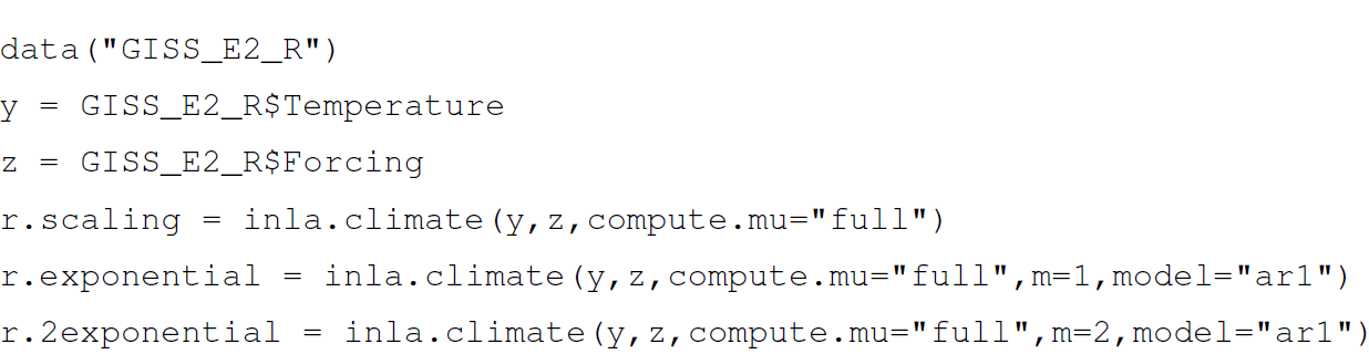
For comparison, we apply the same approach to estimate the given marginal posterior distributions under the assumption of an exponential response function in Eq. (3). In this case, the discretized unforced response described in Eq. (4) is an AR(1) process. More generally, the discretized response functions corresponding to Eq. (6) are a weighted sum of m AR(1) processes. Notice that a mixture of a few AR(1) processes will in general have short-range dependence properties, while the approximation in Eq. (17) is constructed to exhibit the long-range dependency structure of fGn. Using the scale-invariant response function or the exponential response functions corresponding to the one- and two-box models, we can compute the marginal posterior means and 95 % credible intervals for each μi. The results are shown in Fig. 2. The marginal posterior means are very similar. However, we observe significantly wider credible intervals for the model using the single-exponential response function. The larger uncertainty suggests that a smaller portion of the variance is explained by the unforced climate variability, leaving more of the variation to be explained by the response to the known forcing. Using the INLA.climate package, we obtain full inference in seconds on a personal computer. The code to run the example is as follows.
3.2 Temperature predictions for Representative Concentration Pathway trajectories
Once trained on historical temperature and forcing data, the response model can easily be used to obtain temperature predictions for different future forcing scenarios. Here, we present global temperature predictions for the years 2016 to 2100 based on the HadCRUT4 temperature data and the greenhouse gas component of the Hansen forcing data for 1850 to 2015. For future forcing, we use the Representative Concentration Pathways (RCPs) RCP2.6 (van Vuuren et al., 2007), RCP4.5 (Clarke et al., 2007; Smith and Wigley, 2006; Wise et al., 2009), RCP6 (Fujino et al., 2006; Hijioka et al., 2008), and RCP8.5 (Riahi et al., 2007). These trajectories were first published in 2000 and cover the years 2000 to 2100. In our analyses, we use the RCPs for the year 2016 to the year 2100 and adjust each of them so that the forcing in 2015 equals the greenhouse gas forcing in the Hansen data in 2015. The forcing scenarios are shown in Fig. 3.
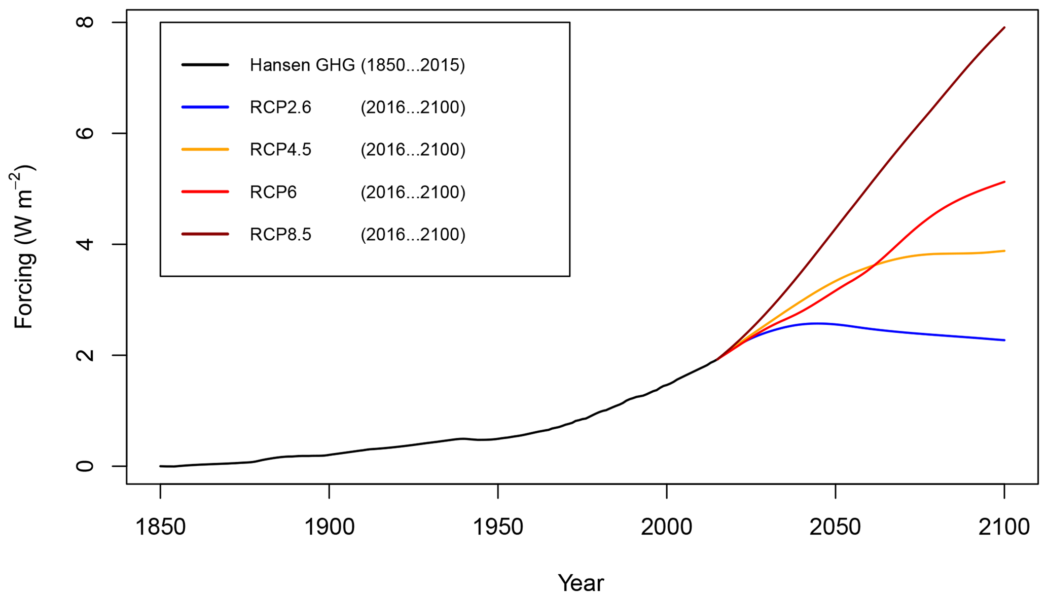
Figure 3The greenhouse gas component of the Hansen forcing (black) followed by the RCP2.6 (blue), RCP4.5 (orange), RCP6 (red), and RCP8.5 (dark red) forcing scenarios.
Prediction is carried out using INLA.climate by appending the future scenario to the forcing of the past . The package automatically replaces missing observations with NA values and give predictions for these based on the model fitted to the observed data.
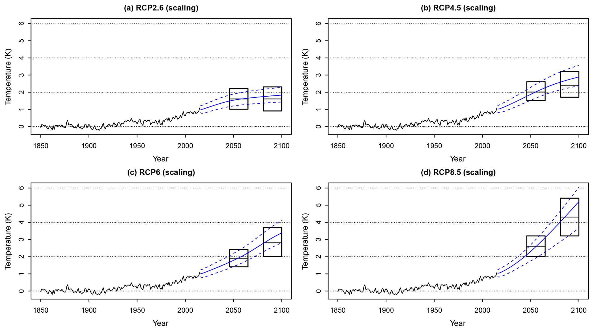
Figure 4Panels (a)–(d) describe the marginal posterior means and 95 % credible intervals of the predicted temperature response to future forcing according to the RCP2.6, RCP4.5, RCP6, and RCP8.5 trajectories, respectively, using a scaling response function. These are compared to the AR5 projections (black boxes).
As in the previous example, we compare the results using the scale-invariant response function versus the exponential response functions corresponding to the one- and two-box models. Training and predictions only take seconds to carry out on a personal computer. Figure 4 shows the marginal posterior means and 95 % credible intervals using the scale-invariant response, while Figs. 5–6 show the corresponding results using the exponential response functions. The figures also show comparisons with the AR5 projections listed in table SPM.2 in IPCC (2013b). We observe that both of the exponential response models seem to fail in describing the persistence in the temperature response and underestimate the global warming increase projections. The predictions obtained using the scale-invariant response function give higher future temperatures estimates, slightly overestimating the AR5 projections.
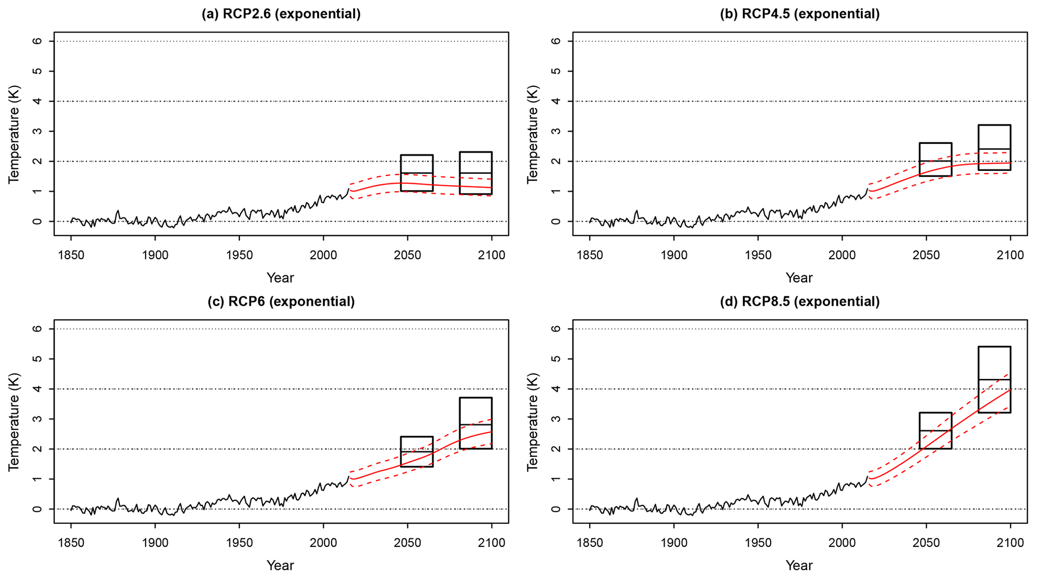
Figure 5Panels (a)–(d) describe the marginal posterior means and 95 % credible intervals of the predicted temperature response to future forcing according to the RCP2.6, RCP4.5, RCP6, and RCP8.5 trajectories, respectively, using a single-exponential response function. These are compared to the AR5 projections (black boxes).
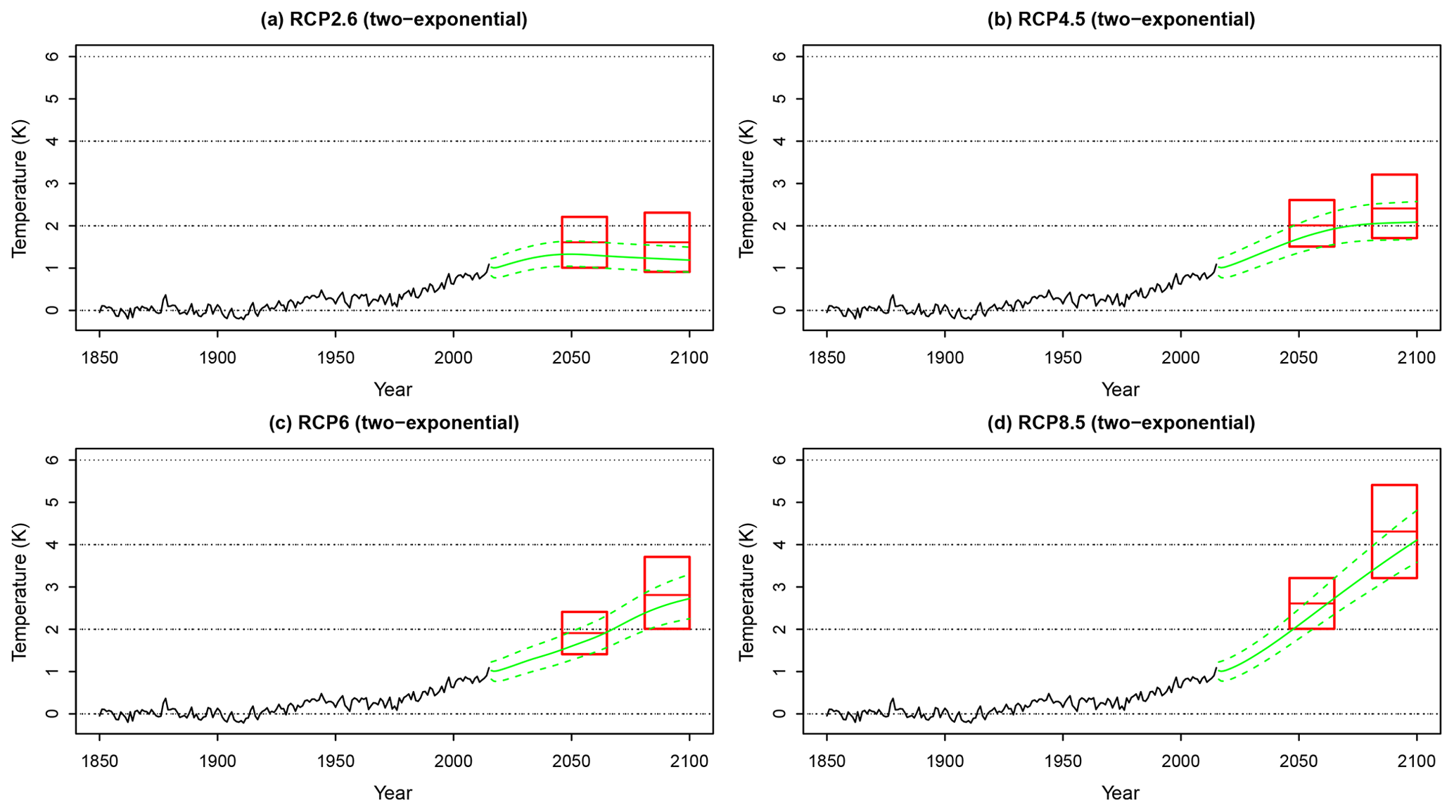
Figure 6Panels (a)–(d) describe the marginal posterior means and 95 % credible intervals of the predicted temperature response to future forcing according to the RCP2.6, RCP4.5, RCP6, and RCP8.5 trajectories, respectively, using a mixture of two-exponential response functions. These are compared to the AR5 projections (black boxes).
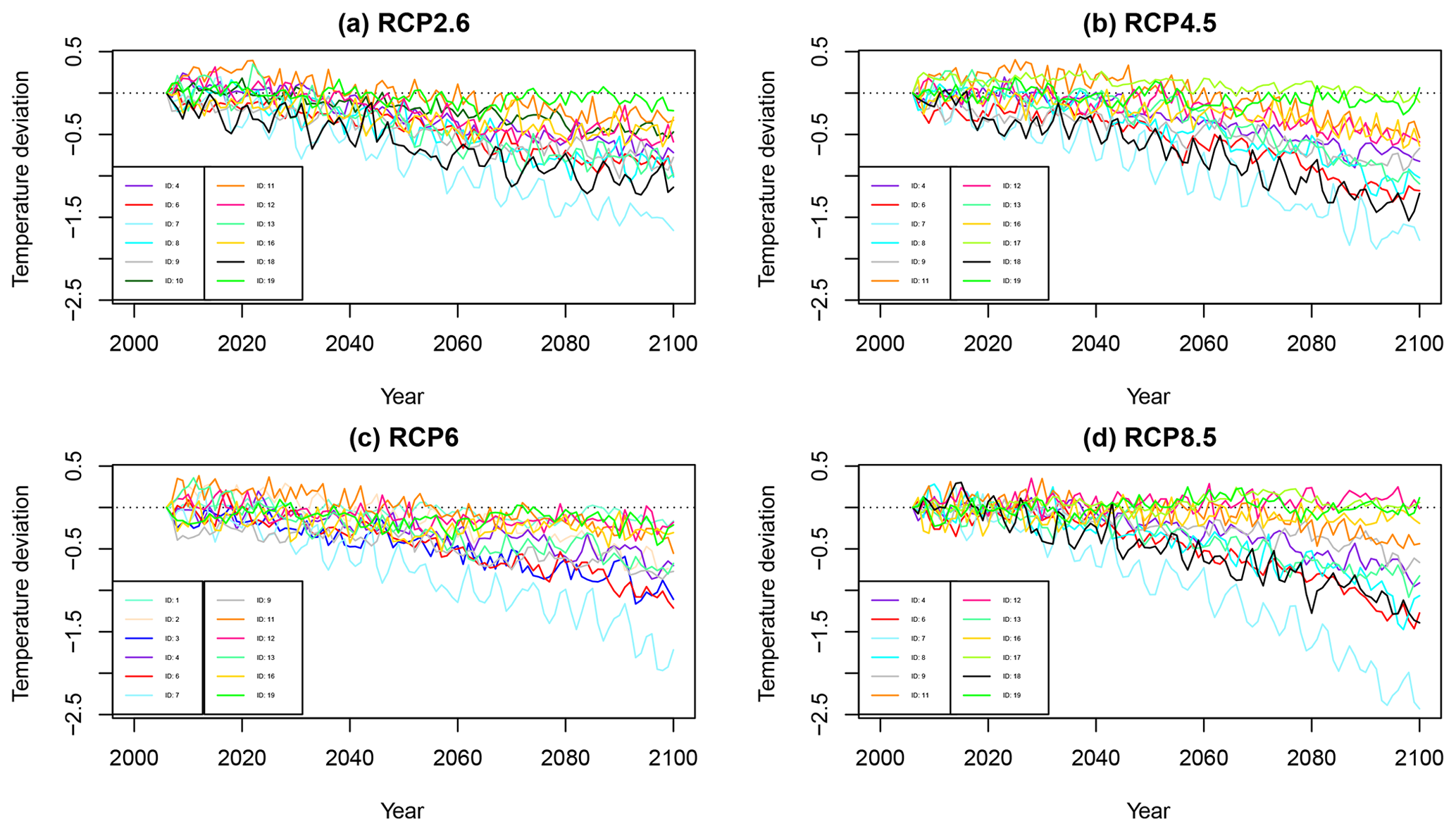
Figure 7Panels (a)–(d) describe the deviations between the predicted marginal posterior means and the predictions obtained from each ESM.
In Fig. 7 we compare the scale-invariant model's temperature projections for RCP scenarios to ESM temperature projections. In this analysis, we tune the statistical model to historical runs of different ESMs in the CMIP5 ensemble. As in the other analyses, we use model-specific forcing for each of the ESMs. Using the same method as for historical forcing, we also estimate model-specific RCP forcing for each of the ESMs and each RCP scenario. From this RCP forcing, and using the estimated parameters, we project GMST under the RCP scenarios and compare with the corresponding projections in the ESMs. Figure 7 shows the differences between the two types of projections. As seen from the figure, there is a negative trend for almost all models and all scenarios, indicating that the predictions made using the statistical model slightly overestimate the temperature increase in the ESMs. This overestimation is not a statistical bias. Instead, it shows that scale invariance is too crude an approximation for several ESMs. One can interpret the differences as a weakness of the scale-free model. However, not all climate models have scaling properties consistent with temperature reconstructions, and it could also reflect the weaknesses of the ESMs.
3.3 Estimating the transient climate response
As a final application, we describe how our suggested method using a scale-invariant response function can be used to estimate the TCR. The TCR is defined as the average temperature response between 60 and 80 years following a gradual CO2 doubling, assuming a 1 % annual increase. In this scenario, the forcing increases linearly according to
Here, is a model-specific coefficient describing the forcing corresponding to a CO2 doubling. We obtain these coefficients from Forster et al. (2013) for all ESMs analyzed in this paper.
The computation of TCR is carried out by inserting the forcing into Eq. (1) and performing the matrix multiplication
where G(H) is the 80×80 matrix with elements defined as in Eq. (10) and . This implies that TCR is computed by
As in Sect. 3.1, the approximate marginal posterior distribution for TCR is obtained by combining INLA with Monte Carlo sampling. We first generate samples from the joint posterior distribution of the model parameters p(θ|ΔT). For each of these samples, we calculate TCR, which then gives the approximate posterior distribution for TCR.
Table 1The average absolute value of the bias, the root mean square error, and the correlation obtained when comparing the marginal posterior mean estimates of the TCR with the TCR obtained directly from the ESMs.
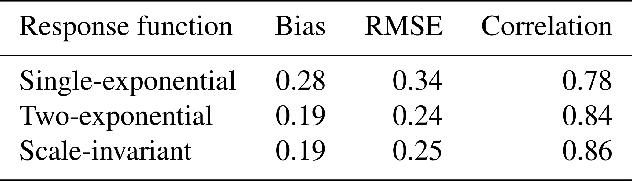
Table 2The Earth system models used in this paper. The table includes ID number, references, time interval, TCR obtained directly from the ESM, and slope coefficient for the forcing corresponding to a CO2 doubling.
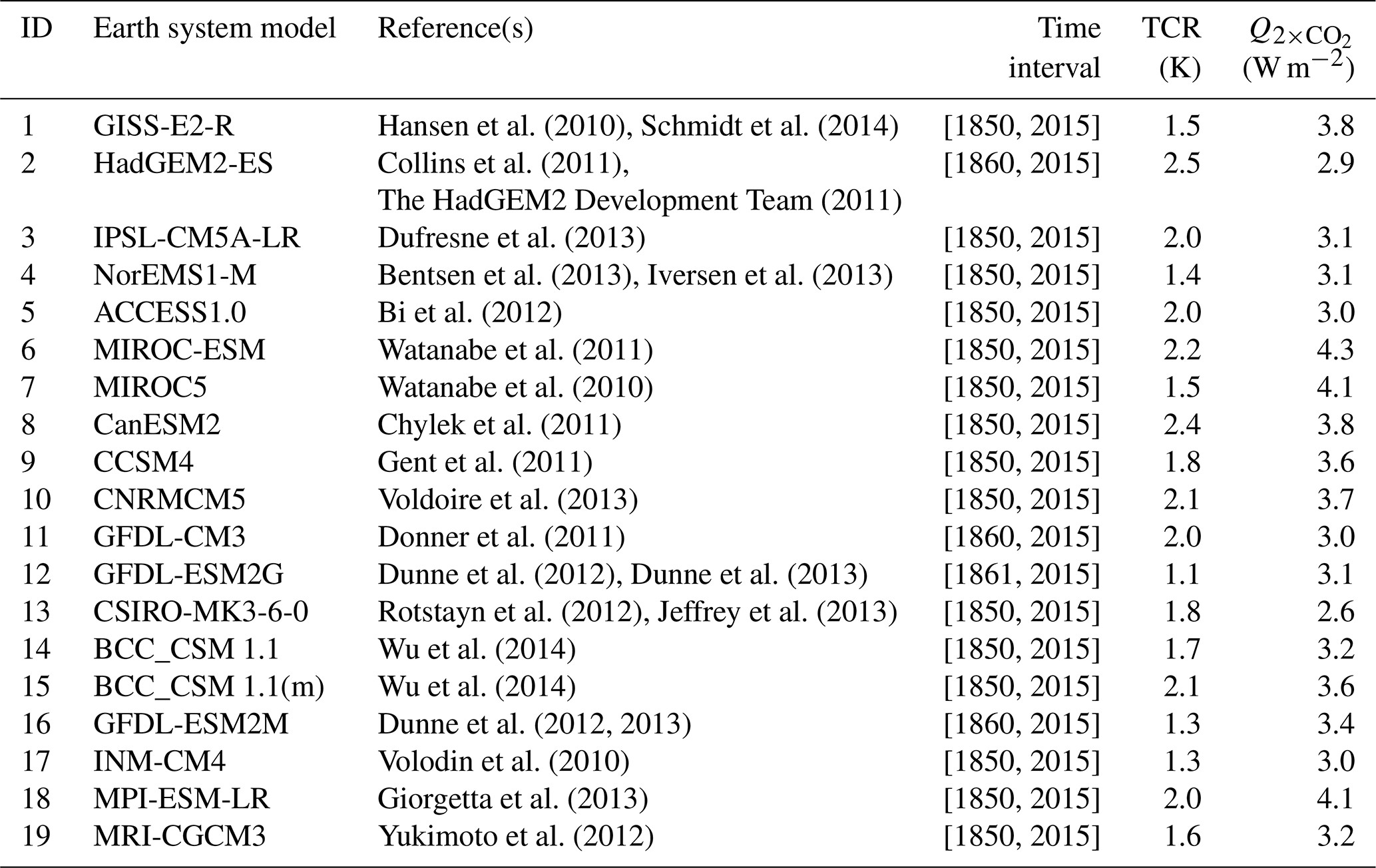
Table 3This table contains marginal posterior means and 95 % credible intervals for the model parameters and the transient climate response obtained from fitting the scale-invariant response model to temperature data from the first nine ESMs.
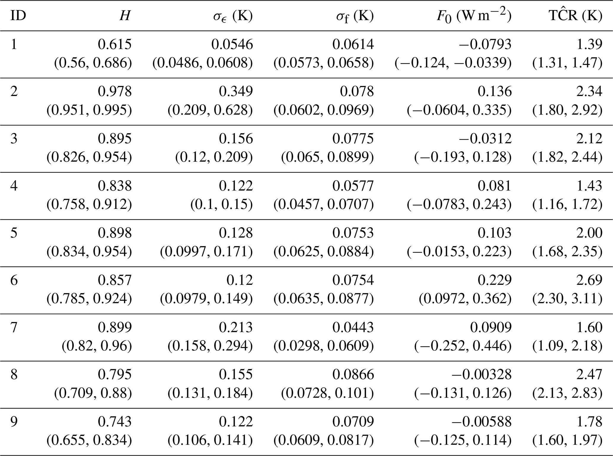
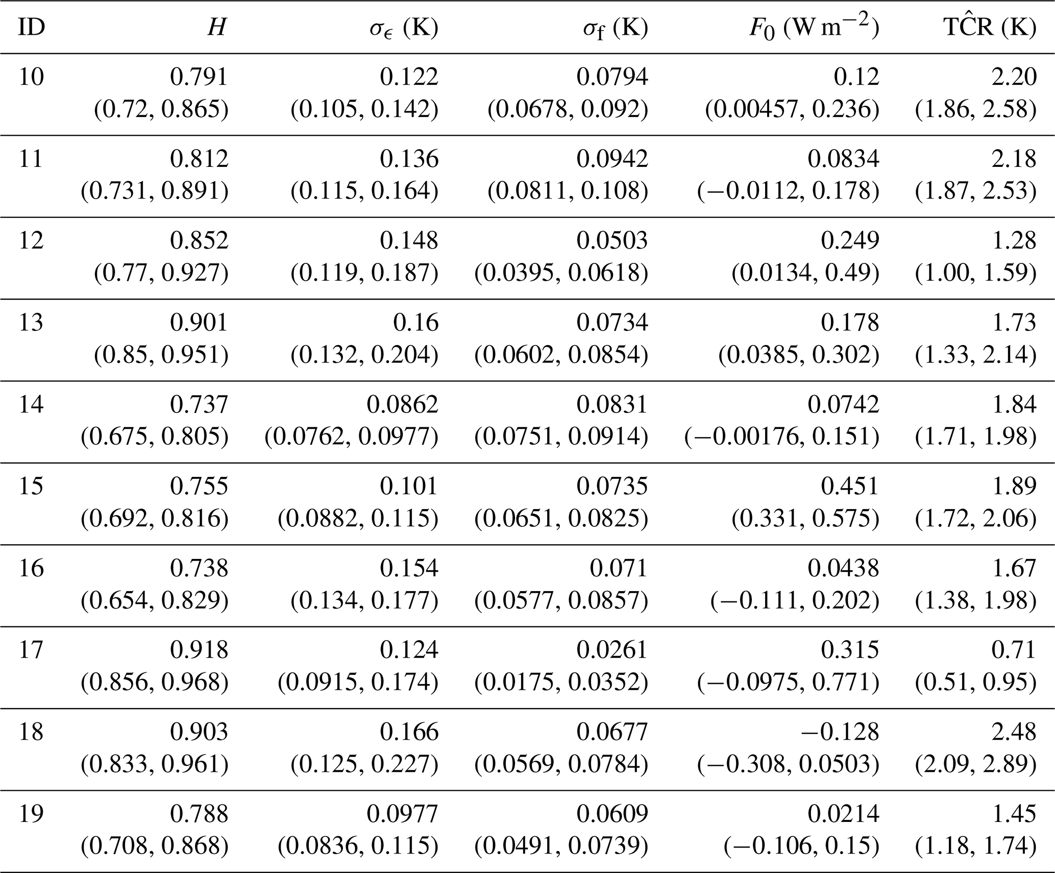
Table 4This table contains marginal posterior means and 95 % credible intervals for the model parameters and the transient climate response obtained from fitting the scale-invariant response model to temperature data from the last 10 ESMs.
For our analyses, we use temperature datasets generated from 19 ESMs in the Coupled Model Intercomparison Project Phase 5 (CMIP5) ensemble; see Table 2. We obtain the forcing by combining the forcing data from Forster et al. (2013) and Hansen et al. (2010) such that the 18-year moving averages of the two are equal. We use the instrumental HadCRUT dataset (Morice et al., 2012), which combines the land temperatures of the CRU dataset (Jones et al., 2012) with the sea surface temperatures of HadSST3 (Kennedy et al., 2011).
To assess the accuracy of the TCR estimations from Eq. (12) we compare the estimates from each of the 19 ESMs with the TCR obtained from the ESMs directly (Forster et al., 2013). Inference is obtained by producing 100 000 Monte Carlo simulations of the TCR. Summary statistics for our model are shown in Tables 3–4, which include the marginal posterior means and 95 % credible intervals for the TCR and the model parameters used to compute it.
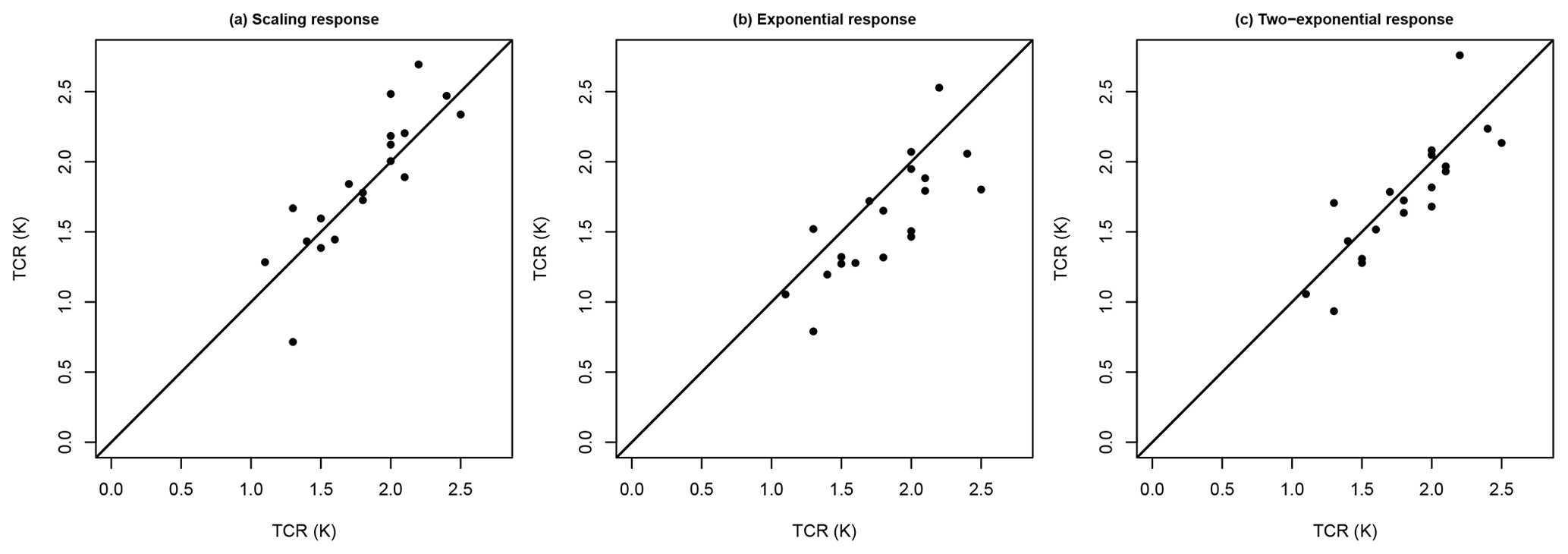
Figure 8Scatter plot of the TCR obtained directly from the 19 ESMs against the corresponding marginal posterior mean estimates when using a scale-invariant response function (a), a single-exponential response function (b), and a two-exponential response function (c).
To assess the approach using the scale-invariant versus the exponential response functions, we compare the posterior mean estimates with the values obtained directly from the ESMs. Specifically, we calculate the average absolute value of the bias, the root mean square error (RMSE), and the correlation between the posterior mean estimates and the TCR values from the ESMs; see Table 1. We observe that the method using the single-exponential response model clearly performs worse than the other two approaches, having higher error and lower correlation with the TCR estimates from the ESMs. The two-exponential response function and the scale-invariant approach perform similarly, with the latter approach showing slightly higher correlation. These two methods have approximately the same average absolute value of the bias, but the two-exponential approach slightly underestimates TCR, while the scale-invariant approach slightly overestimates TCR. This is illustrated by the scatter plots in Fig. 8.
Using INLA.climate, we obtained, for a typical analysis, inference in around 13 s using a scale-invariant response and 35 s using the exponential response functions.
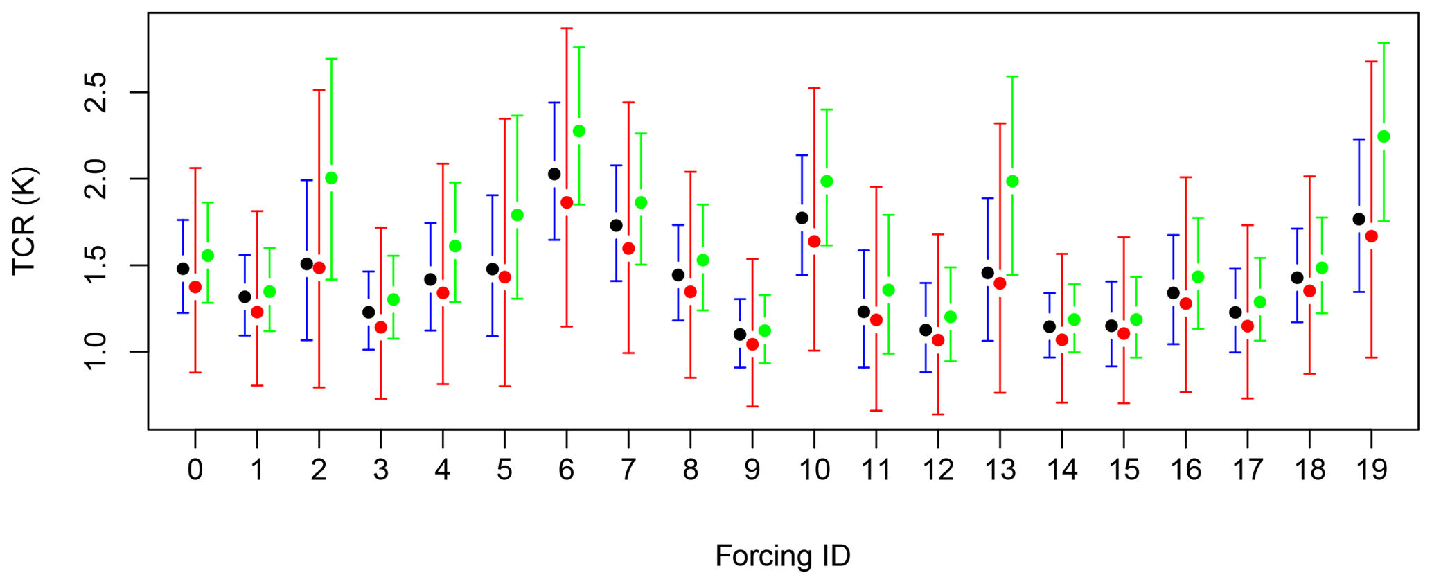
Figure 9The posterior mean estimates and 95 % credible intervals of the historical TCR for all forcing datasets using a scale-invariant (blue), a single-exponential (red), and a two-exponential (green) response function. ID number 0 denotes the Hansen forcing.
To obtain estimates for the TCR of the HadCRUT4 dataset we use 19 different forcing data points associated with the ESMs listed in Table 2 and the Hansen radiative forcing, which we will assign ID number 0. The Monte Carlo simulations are carried out separately for each forcing dataset using 100 000 samples and a forcing slope coefficient W m−2 (IPCC, 2013a).
This is again performed using both the scale-invariant and the exponential response functions.
For the scale-invariant response, the posterior means and credibility intervals of the TCR and the parameters used to compute the TCR for each ESM are shown in Tables 5–6. The marginal posterior mean estimates and 95 % credible intervals for the TCR using all approaches are illustrated in Fig. 9 where we observe wider credible intervals when using a single-exponential response function.
We obtain an estimated posterior distribution for the TCR across all models by aggregating all TCR samples obtained from each analysis, totaling 2 million simulations.
The posterior density is obtained from the Monte Carlo samples using the density function in R. The resulting density function is depicted in Fig. 10, where it is compared with a histogram describing the TCRs obtained directly from the ESMs. We observe a mean of 1.43, 1.35, and 1.61 K and standard deviation of 0.19, 0.40, and 0.40 K when using a scale-invariant, a single-exponential, and a two-exponential response function, respectively.
The given estimates mainly fall in the lower half of the range of TCRs and fail to capture the mode of the histogram. However, since the histogram is generated from only 19 different values of TCR, its form is influenced by the size of the bins. Using bins of width 0.5 K (resulting in three total bins) would describe a more unimodal distribution with a mode in the 1.5–2.0 interval. The posterior distribution obtained from using either a scale-invariant or the exponential response functions is still on the lower side of this.
Table 5This table contains marginal posterior means and 95 % credible intervals for the model parameters and the transient climate response obtained from fitting the scale-invariant response model to the HadCRUT dataset using forcing data from Hansen et al. (2010) (denoted by ID 0) and from the first nine ESMs.
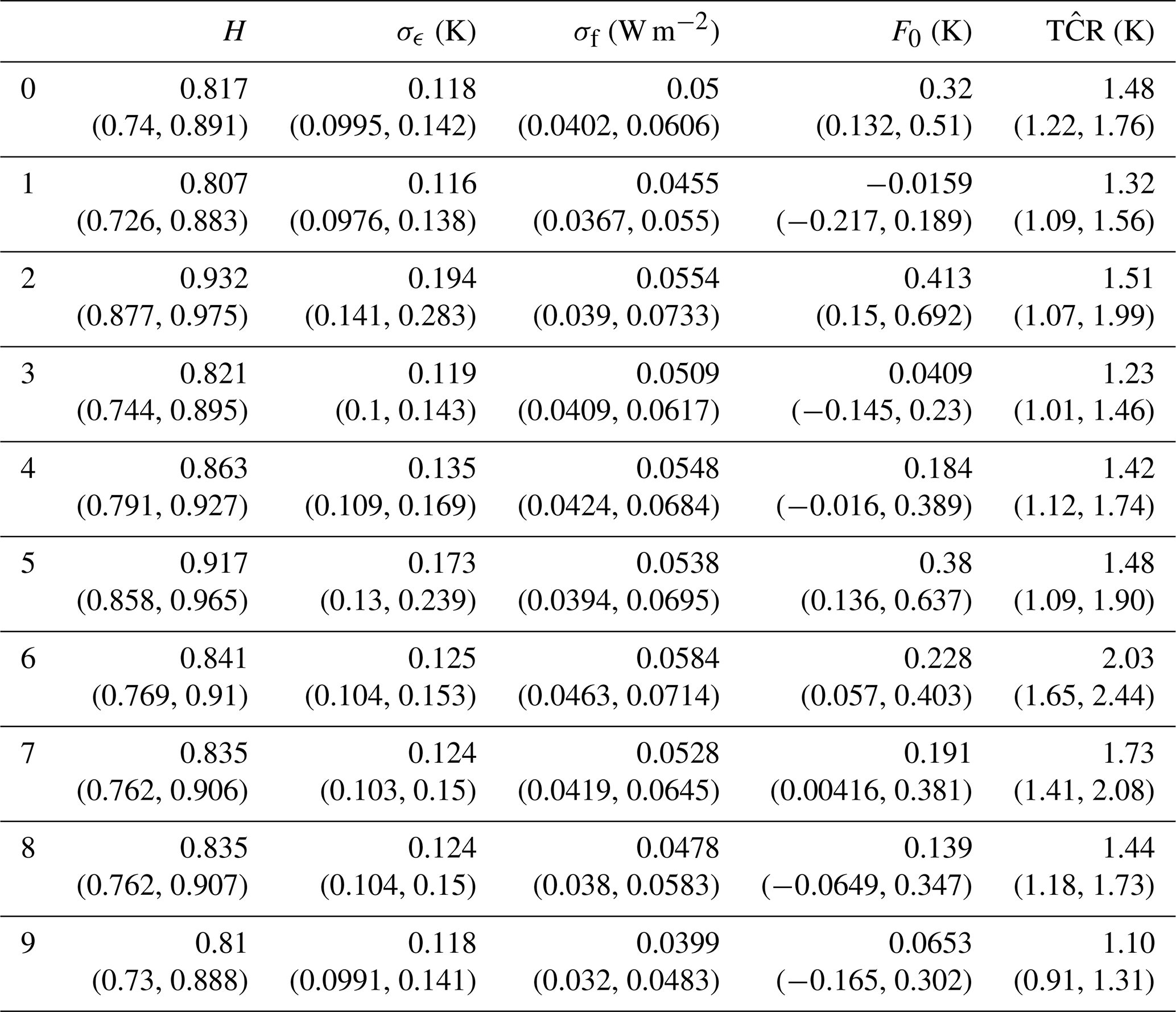
Table 6This table contains marginal posterior means and 95 % credible intervals for the model parameters and the transient climate response obtained from fitting the scale-invariant response model to the HadCRUT dataset using forcing data from the last 10 ESMs.
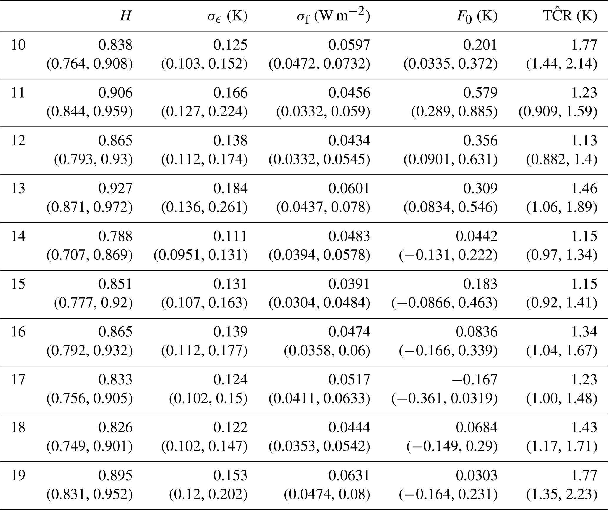
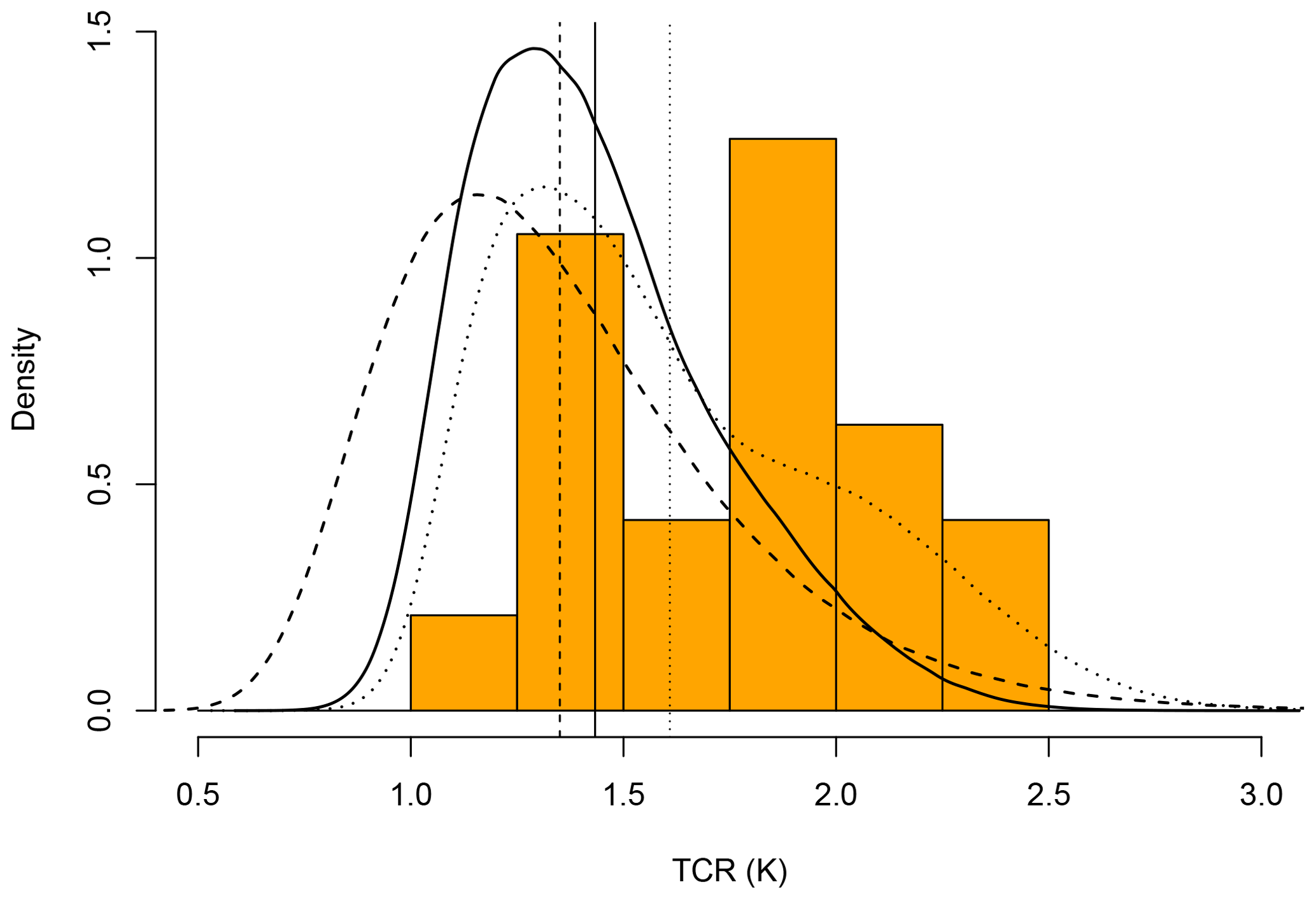
Figure 10Histogram of the TCR obtained from the different ESMs with the posterior density function estimated from the Monte Carlo simulations using a scale-invariant (solid), a single-exponential (dashed), and a two-exponential (dotted) response function. The vertical lines describe the means of the three approaches.
This paper presents a Bayesian formulation to analyze a linear temperature response model to radiative forcing, incorporating long-range temporal dependence using a scale-invariant response function. Computational efficiency is achieved by incorporating the model within
the R-INLA framework and adopting the approximation introduced in Sørbye et al. (2019).
The benefits of this methodology are threefold. First, the model is both accessible and adaptable to more advanced models that require more trends and effects. Second, the approximations ensure low costs in both computational complexity and memory, even for long time series. Third, the method yields full Bayesian inference, giving a full description of the behavior of the time variables and model parameters.
In addition to providing parameter estimates, the model has been used to produce temperature predictions as responses to the four RCP forcing trajectories used to describe future radiative forcing. For comparison, we have also included prediction results using the one-box and two-box energy balance models, giving single-exponential or a mixture of two-exponential response functions, respectively. We observe that the exponential response models underestimate the predicted temperature compared to the projections made by the IPCC. On the other hand, the scale-invariant response models tend to overestimate future temperatures but are overall more accurate than using the exponential response functions.
We further demonstrate that the model can be used to estimate the transient climate response in instrumental data. Our best estimate is that the TCR is 1.43 K with a standard deviation of 0.29 K. This estimate falls right in the middle of the range put forward in the IPCC report (0.8–2.5 K), and the accuracy is consistent with the TCR obtained directly from the ESMs. The presented model has also given coherent estimates for the equilibrium climate sensitivity compared with running ESMs (Rypdal et al., 2018a).
Accurate linear response models for global temperature are essential alternatives to ESMs in studies in which one needs to explore a large number of emission scenarios, and the modeling framework presented here can easily be included in integrated assessment models. Moreover, since the models are invertible, they can efficiently compute forcing scenarios corresponding to given future scenarios for global temperatures. Hence, in combination with linear models for the CO2 response to emissions, they can be used to obtain observation-based estimates of the remaining carbon budget in scenarios in which we reach the goals of the Paris Agreement.
In combination with dedicated ESM experiments, the methods presented in this paper can also be used to estimate global and regional climate sensitivity as a function of background state and timescale. One can use such estimates to study the effect of nonlinear responses across timescales and to obtain insight into how sensitivities and fluctuations change in the vicinity of climate tipping points.
The code and datasets used for this paper are available through the R package INLA.climate, which can be downloaded from https://github.com/eirikmn/INLA.climate (Myrvoll-Nilsen, 2020).
All authors conceived and designed the study; HBF collected data and constructed the modified forcing data.
EMN implemented the model, performed all of the analyses, and developed the R package INLA.climate. HR provided technical support related to R-INLA. EMN, SHS, and MR discussed the results and wrote the paper.
The authors declare that they have no conflict of interest.
The authors thank Kristoffer Rypdal for useful discussions.
This research has been supported by the European Union Horizon 2020 research and innovation program (grant no. 820970).
This paper was edited by Michel Crucifix and reviewed by two anonymous referees.
Annan, J. D. and Hargreaves, J. C.: Using multiple observationally‐based constraints to estimate climate sensitivity, Geophys. Res. Lett., 33, L06704, https://doi.org/10.1029/2005GL025259, 2006. a
Barboza, L. A., Emile-Geay, J., Li, B., and He, W.: Efficient Reconstructions of Common Era Climate via Integrated Nested Laplace Approximations, J. Agr. Biol. Envir. St., 24, 535–554, 2019. a
Bentsen, M., Bethke, I., Debernard, J. B., Iversen, T., Kirkevåg, A., Seland, Ø., Drange, H., Roelandt, C., Seierstad, I. A., Hoose, C., and Kristjánsson, J. E.: The Norwegian Earth System Model, NorESM1-M – Part 1: Description and basic evaluation of the physical climate, Geosci. Model Dev., 6, 687–720, https://doi.org/10.5194/gmd-6-687-2013, 2013. a
Bi, D., Dix, M., Marsland, S., O'Farrell, S., Rashid, H., Uotila, P., Hirst, T., Kowalczyk, E., Golebiewski, M., Sullivan, A., Yan, H., Hannah, N., Franklin, C., Sun, Z., Vohralik, P., Watterson, I., Zhou, X., Fiedler, R., Collier, M., Ma, Y., Noonan, J., Stevens, L., Uhe, P., Zhu, H., Griffies, S., Hill, R., Harris, C., and Puri, K.: The ACCESS coupled model: Description, control climate and evaluation, Aust. Meteorol. Ocean, 63, 41–64, 2012. a
Caldeira, K. and Myhrvold, N. P.: Projections of the pace of warming following an abrupt increase in atmospheric carbon dioxide concentration, Environ. Res. Lett., 8, 034039, https://doi.org/10.1088/1748-9326/8/3/034039, 2013. a
Chylek, P., Li, J., Dubey, M. K., Wang, M., and Lesins, G.: Observed and model simulated 20th century Arctic temperature variability: Canadian Earth System Model CanESM2, Atmos. Chem. Phys. Discuss., 11, 22893–22907, https://doi.org/10.5194/acpd-11-22893-2011, 2011. a
Clarke, L., Edmonds, J., Jacoby, H., Pitcher, H., Reilly, J., and Richels, R.: Scenarios of Greenhouse Gas Emissions and Atmospheric Concentrations, sub-report 2.1A of Synthesis and Assessment Product 2.1 by the U.S. Climate Change Science Program and the Subcommittee on Global Change Research. Department of Energy, Office of Biological & Environmental Research, US Department of Energy Publications, Lincoln, NE, USA, 2007. a
Collins, W. J., Bellouin, N., Doutriaux-Boucher, M., Gedney, N., Halloran, P., Hinton, T., Hughes, J., Jones, C. D., Joshi, M., Liddicoat, S., Martin, G., O'Connor, F., Rae, J., Senior, C., Sitch, S., Totterdell, I., Wiltshire, A., and Woodward, S.: Development and evaluation of an Earth-System model – HadGEM2, Geosci. Model Dev., 4, 1051–1075, https://doi.org/10.5194/gmd-4-1051-2011, 2011. a
Cox, P. M., Huntingford, C., and Williamson, M.: Emergent constraint on equilibrium climate sensitivity from global temperature variability, Nature, 553, 319–322, 2018. a
Donner, L. J., Wyman, B. L., Hemler, R. S., Horowitz, L. W., Ming, Y., Zhao, M., Golaz, J.-C., Ginoux, P., Lin, S.-J., Schwarzkopf, M. D., Austin, J., Alaka, G., Cooke, W. F., Delworth, T. L., Freidenreich, S. M., Gordon, C. T., Griffies, S. M., Held, I. M., Hurlin, W. J., Klein, S. A., Knutson, T. R., Langenhorst, A. R., Lee, H.-C., Lin, Y., Magi, B. I., Malyshev, S. L., Milly, P. C. D., Naik, V., Nath, M. J., Pincus, R., Ploshay, J. J., Ramaswamy, V., Seman, C. J., Shevliakova, E., Sirutis, J. J., Stern, W. F., Stouffer, R. J., Wilson, R. J., Winton, M., Wittenberg, A. T., and Zeng, F.: The Dynamical Core, Physical Parameterizations, and Basic Simulation Characteristics of the Atmospheric Component AM3 of the GFDL Global Coupled Model CM3, J. Climate, 24, 3484–3519, 2011. a
Dufresne, J.-L., Foujols, M.-A., Denvil, S., Caubel, A., Marti, O., Aumont, O., Balkanski, Y., Bekki, S., Bellenger, H., Benshila, R., Bony, S., Bopp, L., Braconnot, P., Brockmann, P., Cadule, P., Cheruy, F., Codron, F., Cozic, A., Cugnet, D., de Noblet, N., Duvel, J.-P., Ethé, C., Fairhead, L., Fichefet, T., Flavoni, S., Friedlingstein, P., Grandpeix, J.-Y., Guez, L., Guilyardi, E., Hauglustaine, D., Hourdin, F., Idelkadi, A., Ghattas, J., Joussaume, S., Kageyama, M., Krinner, G., Labetoulle, S., Lahellec, A., Lefebvre, M.-P., Lefevre, F., Levy, C., Li, Z. X., Lloyd, J., Lott, F., Madec, G., Mancip, M., Marchand, M., Masson, S., Meurdesoif, Y., Mignot, J., Musat, I., Parouty, S., Polcher, J., Rio, C., Schulz, M., Swingedouw, D., Szopa, S., Talandier, C., Terray, P., Viovy, N., and Vuichard, N.: Climate change projections using the IPSL-CM5 Earth System Model: from CMIP3 to CMIP5, Clim. Dynam., 40, 2123–2165, 2013. a
Dunne, J. P., John, J. G., Adcroft, A. J., Griffies, S. M., Hallberg, R. W., Shevliakova, E., Stouffer, R. J., Cooke, W., Dunne, K. A., Harrison, M. J., Krasting, J. P., Malyshev, S. L., Milly, P. C. D., Phillipps, P. J., Sentman, L. T., Samuels, B. L., Spelman, M. J., Winton, M., Wittenberg, A. T., and Zadeh, N.: GFDL's ESM2 Global Coupled Climate–Carbon Earth System Models. Part I: Physical Formulation and Baseline Simulation Characteristics, J. Climate, 25, 6646–6665, 2012. a, b
Dunne, J. P., John, J. G., Shevliakova, E., Stouffer, R. J., Krasting, J. P., Malyshev, S. L., Milly, P. C. D., Sentman, L. T., Adcroft, A. J., Cooke, W., Dunne, K. A., Griffies, S. M., Hallberg, R. W., Harrison, M. J., Levy, H., Wittenberg, A. T., Phillips, P. J., and Zadeh, N.: GFDL's ESM2 Global Coupled Climate-Carbon Earth System Models. Part II: Carbon System Formulation and Baseline Simulation Characteristics, J. Climate, 26, 2247–2267, 2013. a, b
Flato, G. M.: Earth system models: an overview, WIREs Clim. Change, 2, 783–800, 2011. a
Forster, P. M., Andrews, T., Good, P., Gregory, J. M., Jackson, L. S., and Zelinka, M.: Evaluating adjusted forcing and model spread for historical and future scenarios in the CMIP5 generation of climate models, J. Geophys. Res.-Atmos., 118, 1139–1150, 2013. a, b, c
Franzke, C.: Long-Range Dependence and Climate Noise Characteristics of Antarctic Temperature Data, J. Climate, 23, 6074–6081, 2010. a
Fredriksen, H.-B. and Rypdal, K.: Spectral characteristics of instrumental and climate model surface temperatures, J. Climate, 29, 1253–1268, 2016. a
Fredriksen, H.-B. and Rypdal, M.: Long-Range Persistence in Global Surface Temperatures Explained by Linear Multibox Energy Balance Models, J. Climate, 30, 7157–7168, 2017. a, b, c
Fujino, J., Nair, R., Kainuma, M., Masui, T., and Matsuoka, Y.: Multi-gas Mitigation Analysis on Stabilization Scenarios Using Aim Global Model, Energ. J., 27, 343–353, 2006. a
Gent, P. R., Danabasoglu, G., Donner, L. J., Holland, M. M., Hunke, E. C., Jayne, S. R., Lawrence, D. M., Neale, R. B., Rasch, P. J., Vertenstein, M., Worley, P. H., Yang, Z.-L., and Zhang, M.: The Community Climate System Model Version 4, J. Climate, 24, 4973–4991, 2011. a
Geoffroy, O., Saint-Martin, D., Olivié, D. J. L., Voldoire, A., Bellon, G., and Tytéca, S.: Transient climate response in a two-layer energy-balance model. Part I: Analytical solution and parameter calibration using CMIP5 AOGCM experiments, J. Climate, 26, 1841–1857, 2013. a
Giorgetta, M. A., Jungclaus, J., Reick, C. H., Legutke, S., Bader, J., Böttinger, M., Brovkin, V., Crueger, T., Esch, M., Fieg, K., Glushak, K., Gayler, V., Haak, H., Hollweg, H.-D., Ilyina, T., Kinne, S., Kornblueh, L., Matei, D., Mauritsen, T., Mikolajewicz, U., Mueller, W., Notz, D., Pithan, F., Raddatz, T., Rast, S., Redler, R., Roeckner, E., Schmidt, H., Schnur, R., Segschneider, J., Six, K. D., Stockhause, M., Timmreck, C., Wegner, J., Widmann, H., Wieners, K.-H., Claussen, M., Marotzke, J., and Stevens, B.: Climate and carbon cycle changes from 1850 to 2100 in MPI-ESM simulations for the Coupled Model Intercomparison Project phase 5, J. Adv. Model. Earth Syst., 5, 572–597, 2013. a
Hansen, J., Ruedy, R., Sato, M., and Lo, K.: Global surface temperature change, Rev. Geophys., 48, RG4004, https://doi.org/10.1029/2010RG000345, 2010. a, b, c
Hansen, J., Sato, M., Russell, G., and Kharecha, P.: Climate sensitivity, sea level and atmospheric carbon dioxide, Philos. T. Roy. Soc. A, 371, 20120294, https://doi.org/10.1098/rsta.2012.0294, 2013. a
Held, I. M., Winton, M., Takahashi, K., Delworth, T., Zeng, F., and Vallis, G. K.: Probing the fast and slow components of global warming by returning abruptly to preindustrial forcing, J. Climate, 23, 2418–2427, 2010. a
Hijioka, Y., Matsuoka, Y., Nishimoto, H., Masui, T., and Kainuma, M.: Global GHG emissions scenarios under GHG concentration stabilization targets, J. Glob. Environ. Eng., 13, 97–108, 2008. a
Huybers, P. and Curry, W.: Links between annual, Milankovitch and continuum temperature variability, Nature, 441, 329–332, 2005. a
IPCC: Climate Change 2013: The Physical Science Basis. Contribution of Working Group I to the Fifth Assessment Report of the Intergovernmental Panel on Climate Change, edited by: Stocker, T. F., Qin, D., Plattner, G.-K., Tignor, M., Allen, S. K., Boschung, J., Nauels, A., Xia, Y., Bex, V., and Midgley, P. M., Cambridge University Press, Cambridge, UK and New York, NY, USA, 2013a. a
IPCC: Summary for Policymakers, book section SPM, edited by: Stocker, T. F., Qin, D., Plattner, G.-K., Tignor, M., Allen, S. K., Boschung, J., Nauels, A., Xia, Y., Bex, V., and Midgley, P. M., Cambridge University Press, Cambridge, UK and New York, NY, USA, 1–30, 2013b. a
Iversen, T., Bentsen, M., Bethke, I., Debernard, J. B., Kirkevåg, A., Seland, Ø., Drange, H., Kristjansson, J. E., Medhaug, I., Sand, M., and Seierstad, I. A.: The Norwegian Earth System Model, NorESM1-M – Part 2: Climate response and scenario projections, Geosci. Model Dev., 6, 389–415, https://doi.org/10.5194/gmd-6-389-2013, 2013. a
Jeffrey, S. J., Rotstayn, L. D., Collier, M. A., Dravitzki, S. M., Hamalainen, C., Moeseneder, C., Wong, K. K., and Syktus, J.: Australia's CMIP5 submission using the CSIRO-Mk3.6 model, Aust. Meteorol. Ocean, 63, 1–13, 2013. a
Jones, P., Lister, D., Osborn, T., Harpham, C., and Salmon, M. M. C.: Hemispheric and large-scale land-surface air temperature variations: An extensive revision and an update to 2010, J. Geophys. Res., 117, D05127, https://doi.org/10.1029/2011JD017139, 2012. a
Kennedy, J. J., Rayner, N. A., Smith, R. O., Parker, D. E., and Saunby, M.: Reassessing biases and other uncertainties in sea surfacetemperature observations measured in situ since 1850: 2. Biases and homogenization, J. Geophys. Res., 116, D14104, https://doi.org/10.1029/2010JD015218, 2011. a
Köhler, P., Stap, L. B., von der Heydt, A. S., de Boer, B., van de Wal, R. S. W., and Bloch‐Johnson, J.: A State‐Dependent Quantification of Climate Sensitivity Based on Paleodata of the Last 2.1 Million Years, Paleoceanography, 32, 1102–1114, 2017. a
Lovejoy, S. and Schertzer, D.: The Weather and Climate: Emergent Laws and Multifractal Cascades, Cambridge University Press. Cambridge, UK, 2013. a
Martins, T. G., Simpson, D., Lindgren, F., and Rue, H.: Bayesian computing with INLA: New features, Comput. Stat. Data Anal., 67, 68–83, 2013. a
Morice, C., Kennedy, J., Rayner, N., and Jones, P.: Quantifying uncertainties in global and regional temperature change using an ensemble of observational estimates: The Hadcrut4 data set, J. Geophys. Res., 117, D08101, https://doi.org/10.1029/2011JD017187, 2012. a
Myrvoll-Nilsen, E.: INLA.climate, available at: https://github.com/eirikmn/INLA.climate, last access: 11 February 2020. a
Qu, X., Hall, A., and DeAngelis, A. M.: On the Emergent Constraints of Climate Sensitivity, J. Climate, 31, 863–875, 2018. a
Riahi, K., Grübler, A., and Nakicenovic, N.: Scenarios of long-term socio-economic and environmental development under climate stabilization, greenhouse Gases – Integrated Assessment, Technol. Forecast. Soc. Change, 74, 887–935, 2007. a
Robert, C. and Casella, G.: Monte Carlo Statistical Methods, 1 edn., Springer-Verlag New York, USA, 1999. a
Rotstayn, L. D., Jeffrey, S. J., Collier, M. A., Dravitzki, S. M., Hirst, A. C., Syktus, J. I., and Wong, K. K.: Aerosol- and greenhouse gas-induced changes in summer rainfall and circulation in the Australasian region: a study using single-forcing climate simulations, Atmos. Chem. Phys., 12, 6377–6404, https://doi.org/10.5194/acp-12-6377-2012, 2012. a
Rue, H. and Held, L.: Gaussian Markov Random Fields: Theory And Applications (Monographs on Statistics and Applied Probability, Chapman and Hall-CRC Press, London, UK, 2005. a
Rue, H., Martino, S., and Chopin, N.: Approximate Bayesian inference for latent Gaussian models using integrated nested Laplace approximations (with discussion), J. R. Stat. Soc. Ser. B, 71, 319–392, 2009. a, b, c
Rue, H., Riebler, A., Sørbye, S. H., Illian, J. B., Simpson, D. P., and Lindgren, F. K.: Bayesian Computing with INLA: A Review, Annu. Rev. Stat. Appl., 4, 395–421, 2017. a, b
Rybski, D., Bunde, A., Havlin, S., and von Storch, H.: Long-term persistence in climate and the detection problem, Geophys. Res. Lett., 33, L06718, https://doi.org/10.1029/2005GL025591, 2006. a
Rypdal, K.: Global temperature response to radiative forcing: Solar cycle versus volcanic eruptions, J. Geophys. Res., 117, D06115, https://doi.org/10.1029/2011JD017283, 2012. a
Rypdal, K., Rypdal, M., and Fredriksen, H.-B.: Spatiotemporal long-range persistence in earth's temperature field: Analysis of stochastic-diffusive energy balance models, J. Climate, 28, 8379–8395, 2015. a
Rypdal, M. and Rypdal, K.: Long-Memory Effects in Linear Response Models of Earth's Temperature and Implications for Future Global Warming, J. Climate, 27, 5240–5258, 2014. a, b, c, d
Rypdal, M. and Rypdal, K.: Late Quaternary temperature variability described as abrupt transitions on a 1∕f noise background, Earth Syst. Dynam., 7, 281–293, https://doi.org/10.5194/esd-7-281-2016, 2016. a
Rypdal, M., Fredriksen, H.-B., Myrvoll-Nilsen, E., Rypdal, K., and Sørbye, S. H.: Emergent Scale Invariance and Climate Sensitivity, Climate, 6, 93, https://doi.org/10.3390/cli6040093, 2018a. a, b, c
Rypdal, M., Fredriksen, H.-B., Rypdal, K., and Steene, R. J.: Emergent constraints on climate sensitivity, Nature, 563, E4–E5, 2018b. a
Schmidt, G. A., Kelley, M., Nazarenko, L., Ruedy, R., Russell, G. L., Aleinov, I., Bauer, M., Bauer, S. E., Bhat, M. K., Bleck, R., Canuto, V., Chen, Y.-H., Cheng, Y., Clune, T. L., Del Genio, A., de Fainchtein, R., Faluvegi, G., Hansen, J. E., Healy, R. J., Kiang, N. Y., Koch, D., Lacis, A. A., LeGrande, A. N., Lerner, J., Lo, K. K., Matthews, E. E., Menon, S., Miller, R. L., Oinas, V., Oloso, A. O., Perlwitz, J. P., Puma, M. J., Putman, W. M., Rind, D., Romanou, A., Sato, M., Shindell, D. T., Sun, S., Syed, R. A., Tausnev, N., Tsigaridis, K., Unger, N., Voulgarakis, A., Yao, M.-S., and Zhang, J.: Configuration and assessment of the GISS ModelE2 contributions to the CMIP5 archive, J. Adv. Model. Earth Syst., 6, 141–184, https://doi.org/10.1002/2013MS000265, 2014. a, b
Simpson, D., Rue, H., Riebler, A., Martins, T. G., and Sørbye, S. H.: Penalising Model Component Complexity: A Principled, Practical Approach to Constructing Priors, Stat. Sci., 32, 1–28, 2017. a
Smith, S. J. and Wigley, T.: Multi-Gas Forcing Stabilization with Minicam, Energ. J., 27, 373–391, 2006. a
Sørbye, S. and Rue, H.: Fractional Gaussian noise: Prior specification and model comparison, Environmetrics, 29, e2457, https://doi.org/10.1002/env.2457, 2018. a
Sørbye, S. H., Myrvoll-Nilsen, E., and Rue, H.: An approximate fractional Gaussian noise model with 𝒪(n) computational cost, Stat. Comput., 29, 821–833, 2019. a, b
The HadGEM2 Development Team: Martin, G. M., Bellouin, N., Collins, W. J., Culverwell, I. D., Halloran, P. R., Hardiman, S. C., Hinton, T. J., Jones, C. D., McDonald, R. E., McLaren, A. J., O'Connor, F. M., Roberts, M. J., Rodriguez, J. M., Woodward, S., Best, M. J., Brooks, M. E., Brown, A. R., Butchart, N., Dearden, C., Derbyshire, S. H., Dharssi, I., Doutriaux-Boucher, M., Edwards, J. M., Falloon, P. D., Gedney, N., Gray, L. J., Hewitt, H. T., Hobson, M., Huddleston, M. R., Hughes, J., Ineson, S., Ingram, W. J., James, P. M., Johns, T. C., Johnson, C. E., Jones, A., Jones, C. P., Joshi, M. M., Keen, A. B., Liddicoat, S., Lock, A. P., Maidens, A. V., Manners, J. C., Milton, S. F., Rae, J. G. L., Ridley, J. K., Sellar, A., Senior, C. A., Totterdell, I. J., Verhoef, A., Vidale, P. L., and Wiltshire, A.: The HadGEM2 family of Met Office Unified Model climate configurations, Geosci. Model Dev., 4, 723–757, https://doi.org/10.5194/gmd-4-723-2011, 2011. a
Tierney, L. and Kadane, J. B.: Accurate Approximations for Posterior Moments and Marginal Densities, J. Am. Stat. Assoc., 81, 82–86, 1986. a
van Vuuren, D. P., den Elzen, M. G. J., Lucas, P. L., Eickhout, B., Strengers, B. J., van Ruijven, B., Wonink, S., and van Houdt, R.: Stabilizing greenhouse gas concentrations at low levels: an assessment of reduction strategies and costs, Climatic Change, 81, 119–159, 2007. a
Voldoire, A., Sanchez-Gomez, E., Salas y Mélia, D., Decharme, B., Cassou, C., Sénési, S., Valcke, S., Beau, I., Alias, A., Chevallier, M., Déqué, M., Deshayes, J., Douville, H., Fernandez, E., Madec, G., Maisonnave, E., Moine, M.-P., Planton, S., Saint-Martin, D., Szopa, S., Tyteca, S., Alkama, R., Belamari, S., Braun, A., Coquart, L., and Chauvin, F.: The CNRM-CM5.1 global climate model: description and basic evaluation, Clim. Dynam., 40, 2091–2121, 2013. a
Volodin, E. M., Dianskii, N. A., and Gusev, A. V.: Simulating present-day climate with the INMCM4.0 coupled model of the atmospheric and oceanic general circulations, Izv. Atmos. Ocean Phy.+, 46, 414–431, 2010. a
von der Heydt, A. S. and Ashwin, P.: State dependence of climate sensitivity: attractor constraints and palaeoclimate regimes, Dyn. Stat. Clim. Syst., 1, 1–21, 2017. a
Watanabe, M., Suzuki, T., Oâishi, R., Komuro, Y., Watanabe, S., Emori, S., Takemura, T., Chikira, M., Ogura, T., Sekiguchi, M., Takata, K., Yamazaki, D., Yokohata, T., Nozawa, T., Hasumi, H., Tatebe, H., and Kimoto, M.: Improved Climate Simulation by MIROC5: Mean States, Variability, and Climate Sensitivity, J. Climate, 23, 6312–6335, 2010. a
Watanabe, S., Hajima, T., Sudo, K., Nagashima, T., Takemura, T., Okajima, H., Nozawa, T., Kawase, H., Abe, M., Yokohata, T., Ise, T., Sato, H., Kato, E., Takata, K., Emori, S., and Kawamiya, M.: MIROC-ESM 2010: model description and basic results of CMIP5-20c3m experiments, Geosci. Model Dev., 4, 845–872, https://doi.org/10.5194/gmd-4-845-2011, 2011. a
Wise, M., Calvin, K., Thomson, A., Clarke, L., Bond-Lamberty, B., Sands, R., Smith, S. J., Janetos, A., and Edmonds, J.: Implications of Limiting CO2 Concentrations for Land Use and Energy, Science, 324, 1183–1186, 2009. a
Wu, T., Song, L., Li, W., Wang, Z., Zhang, H., Xin, X., Zhang, Y., Zhang, L., Li, J., Wu, F., Liu, Y., Zhang, F., Shi, X., Chu, M., Zhang, J., Fang, Y., Wang, F., Lu, Y., Liu, X., Wei, M., Liu, Q., Zhou, W., Dong, M., Zhao, Q., Ji, J., Li, L., and Zhou, M.: An overview of BCC climate system model development and application for climate change studies, J. Meteorol. Res., 28, 34–56, 2014. a, b
Yukimoto, S., Adachi, Y., Hosaka, M., Sakami, T., Yoshimura, H., Hirabara, M., Tanaka, T. Y., Shindo, E., Tsujino, H., Deushi, M., Mizuta, R., Yabu, S., Obata, A., Nakano, H., Koshiro, T., Ose, T., and Kitoh, A.: A New Global Climate Model of the Meteorological Research Institute: MRI-CGCM3 – Model Description and Basic Performance, J. Meteorol. Soc. Jpn. Ser. II, 90A, 23–64, 2012. a