the Creative Commons Attribution 4.0 License.
the Creative Commons Attribution 4.0 License.
 | 20 Mar 2020
Back to the future II: tidal evolution of four supercontinent scenarios
J. A. Mattias Green
Joao C. Duarte
The Earth is currently 180 Myr into a supercontinent cycle that began with the break-up of Pangaea and which will end around 200–250 Myr (million years) in the future, as the next supercontinent forms. As the continents move around the planet they change the geometry of ocean basins, and thereby modify their resonant properties. In doing so, oceans move through tidal resonance, causing the global tides to be profoundly affected. Here, we use a dedicated and established global tidal model to simulate the evolution of tides during four future supercontinent scenarios. We show that the number of tidal resonances on Earth varies between one and five in a supercontinent cycle and that they last for no longer than 20 Myr. They occur in opening basins after about 140–180 Myr, an age equivalent to the present-day Atlantic Ocean, which is near resonance for the dominating semi-diurnal tide. They also occur when an ocean basin is closing, highlighting that within its lifetime, a large ocean basin – its history described by the Wilson cycle – may go through two resonances: one when opening and one when closing. The results further support the existence of a super-tidal cycle associated with the supercontinent cycle and gives a deep-time proxy for global tidal energetics.
- Article
(6561 KB) -
Supplement
(73804 KB) - BibTeX
- EndNote


The continents have coalesced into supercontinents and then dispersed several times in Earth's history in a process known as the supercontinent cycle (Nance et al., 1988). While the cycle has an irregular period (Bradley, 2011), the break-up and reformation typically occurs over 500–600 Myr (Nance et al., 2013; Davies et al., 2018; Yoshida and Santosh, 2017, 2018). Pangaea was the latest supercontinent to exist on Earth, forming ∼300 Ma ago, and breaking up around 180 Ma ago, thus initiating the current supercontinent cycle (Scotese, 1991; Golonka, 2007). Another supercontinent should therefore form within the next 200–300 Myr (e.g. Scotese, 2003; Yoshida, 2016; Yoshida and Santosh, 2011, 2017; Duarte et al., 2018; Davies et al., 2018).
The supercontinent cycle is believed to be an effect of plate tectonics and mantle convection (Torsvik, 2010, 2016; Pastor-Galan, 2018), and the break-up and accretion of supercontinents are a consequence of the opening and closing of ocean basins (Wilson, 1966; Conrad and Lithgow-Bertelloni, 2002). The life cycle of each ocean basin is known as the Wilson cycle. A supercontinent cycle may be comprised of more than one Wilson cycle, as several oceans may open and close between the break-up and reformation of a supercontinent (e.g. Hatton, 1997; Murphy and Nance, 2003; Burke, 2011; Duarte et al., 2018; Davies et al., 2018). As ocean basins evolve during the progression of the Wilson cycle (and associated supercontinent cycle), the energetics of the tides within the basins also change (Kagan, 1997; Green et al., 2017). Green et al. (2017, 2018) simulated the evolution of tides from the break-up of Pangaea until the formation of a future supercontinent, thus spanning a whole supercontinent cycle, and found a link between Wilson cycles and tides. They also found that the unusually large present-day tides in the Atlantic, generated because of the near-resonant state of the basin (Platzman, 1975; Egbert et al., 2004; Green, 2010; Arbic and Garrett, 2010), have only been present for the past 1 Myr. However, because the Atlantic is still spreading apart, it will eventually become too wide to sustain resonant tides in the near (geological) future. However, when exactly will this happen, and is it possible that while the continents diverge and converge, other basins will reach the right size to become resonant?
The initial simulation of deep-time future tides by Green et al. (2018) used a scenario of the Earth's tectonic future presented by Duarte et al. (2018) and strengthened the proof-of-concept for the existence of a super-tidal cycle associated with the supercontinent cycle. Their simulations were done using 50–100 Myr intervals between simulations. They acknowledged that this was not long enough to resolve details of the future tidal maxima, including their duration. In this work, we therefore revisit the future evolution of Earth's tides by simulating the tide at 20 Myr intervals during the four different tectonic modes of supercontinent formation summarized by Davies et al. (2018): Pangaea Ultima (based on Scotese, 2003), Novopangaea (Nield, 2007), Aurica (Duarte et al., 2018), and Amasia (based on Mitchell et al., 2012). Pangaea Ultima is a scenario governed by the closing of the Atlantic – an interior ocean – leading to the reformation of a distorted Pangaea (Murphy and Nance 2003, 2008, call this “closure through introversion”). Novopangaea, in contrast, is dominated by the closing of the Pacific Ocean – an exterior ocean – and the formation of a new supercontinent at the antipodes of Pangaea (this is closure through extroversion; Murphy and Nance, 2003). Aurica is a scenario in which the Atlantic and the Pacific close simultaneously and a new ocean opens across Siberia, Mongolia, and India, bisecting Asia (a combination scenario in which two oceans close, one by introversion and another by extroversion; Murphy and Nance, 2005; Duarte et al., 2018). Finally, in the Amasia scenario, the continents gather at the North Pole, 90∘ from Pangaea (this is known as orthoversion; Mitchell et al., 2012). Every scenario has the potential to develop different tidal resonances in different ocean basins at different stages in each ocean's evolution. We focus here on identifying the timing of the occurrence of resonant basins, and on mapping the large-scale evolution of tidal amplitudes and tidal energy dissipation rates in each of the investigated scenarios. We were particularly interested in understanding how common the resonant super-tidal states are, for how long they last, and their relationship with the Wilson cycle.
2.1 Tidal modelling
The future tide was simulated using the Oregon State University Tidal Inversion Software, OTIS, which has been extensively used to simulate global-scale tides of the past, present, and future (Egbert et al., 2004; Green, 2010; Green and Huber, 2013; Wilmes and Green, 2014; Green et al., 2017, 2018). OTIS was benchmarked against other software that simulate global tides and was shown to perform well (Stammer et al., 2014). It provides a solution to the linearized shallow water equations (Egbert et al., 2004):
Here, U is the tidal volume transport vector defined as uh, where u is the horizontal velocity vector and h the water depth, f is the Coriolis parameter, g the acceleration due to gravity, η the sea surface elevation, ηSAL the self-attraction and loading elevation, ηEQ the elevation of the equilibrium tide, and F the energy dissipation term. The latter is defined as , where parameterizes energy due to bed friction using a drag coefficient, Cd =0.003, and Fw=CU represents losses due to tidal conversion. The conversion coefficient, C, is based on Zaron and Egbert (2006) and modified by Green and Huber (2013), computed from
In Eq. (3) γ=50 is a dimensionless scaling factor accounting for unresolved bathymetric roughness, NH is the buoyancy frequency (N) at seabed, is the vertically averaged buoyancy frequency, and ω is the frequency of the M2 tidal constituent, the only constituent analysed here. The buoyancy frequency, N, is based on a statistical fit to present-day climatology (Zaron and Egbert, 2006) and given by , where z is the vertical coordinate counted positively upwards from the sea floor. We did not change N throughout the simulations because the stratification in the future oceans is yet to be quantified.
Each run simulated 14 d, of which 5 d were used for harmonic analysis of the tide. The model output consists of amplitudes and phases of the sea surface elevations and transports, which was used to compute tidal dissipation rates, D, as the difference between the time average of the work done by the tide generating force (W) and the divergence of the horizontal energy flux (P; see Egbert and Ray, 2001, for details):
where W and P are given by
The orbital configuration of the Earth–Moon system, and thereby the tidal and lunar forcing was not changed during the future simulation. The difference in tidal period (+0.11 h) and lunar forcing (−3 %) that occurs after 250 Myr was applied to a sensitivity simulation, which found that the altered parameters do not affect the results sufficiently to warrant changing the values from present day.
2.2 Mapping of future tectonic scenarios
We coupled the kinematic tectonic maps produced by Davies et al. (2018) with OTIS at incremental steps of 20 Myr by using the tectonic maps as boundary conditions in the tidal model. The maps were produced using GPlates, a software specifically designed for the visualization and manipulation of tectonic plates and continents (e.g. Qin et al., 2012; Müller et al., 2018). We used GPlates to digitize and animate a high-resolution representation of present-day continental shelves and coastline (with no ice cover), created from the NOAA ETOPO1 global relief model of the Earth (see Amante and Eakins, 2009 for details). For simplification purposes, shelf extents are kept for the full duration of the scenarios. The continental polygons do not deform, though some overlap is allowed between their margins, to simulate rudimentary continental collision and shortening. Intracontinental break-up and rifting were introduced in three of the scenarios, allowing new ocean basins to form. No continental shelves were extrapolated along the coastlines of these newly formed basins' margins. For more details about the construction of the tectonic scenarios and the respective maps, see Davies et al. (2018).
The resulting maps were then given an artificial land mask 2∘ wide on both poles to allow for numerical convergence (simulations with equilibrium tides near the poles in Green et al., 2017, 2018, did not change the results there), and were constrained to a horizontal resolution of 0.25∘ in both latitude and longitude. They were then assigned a simplified bathymetry; continental shelves were set a depth of 150 m, and mid-ocean ridges were assigned a depth of 1600 m at the crest point and deepening to the abyssal plains within a width of 5∘. Subduction trenches were made 5800 m deep. The depth of the abyssal plains in the maps changes dynamically to retain present-day ocean volume throughout the scenarios. This allows the tidal results of future simulations to be comparable to a present-day simulation, which was tested against real-world tidal observations.
To test the accuracy of our results, we produced and used two present-day bathymetries. The first – a present-day control – is based on version 13 of the Smith and Sandwell bathymetry (Smith and Sandwell, 1997; https://topex.ucsd.edu/marine_topo/, last access: 3 June 2019). A second map was then produced – the present-day degenerate bathymetry – which included a bathymetry created by using the depth values and the method described for the future slices (see Fig. 1 and the corresponding description in Sect. 2.2).
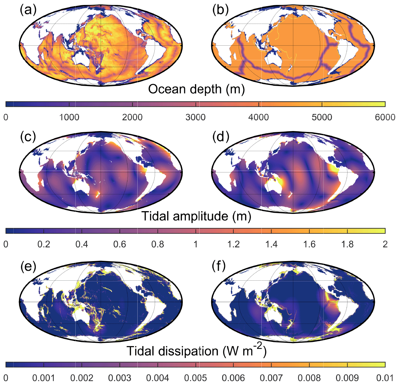
Figure 1(a) The PD bathymetry in m. Panel (b) is the same as (a) but for the degenerate PD bathymetry (see text for details). (c–d) The simulated M2 amplitudes (in m) for the control PD (c) and degenerate PD (d) bathymetries. Note that the colour scale saturates at 2 m. Panels (e–f) are the same as (c)–(d) but show M2 dissipation rates in Wm−2.
The tidal amplitude results for the present-day control simulation (Fig. 1c), when compared to the TPX09 satellite altimetry constrained tidal solution (Egbert and Erofeeva, 2002; https://www.tpxo.net/global/tpxo9-atlas, last access: 28 May 2019), produced an rms error of ±12 cm. Comparing the present-day degenerate simulation (Fig. 1d) results to TPXO9 resulted in an rms error of 13 cm. This is consistent with previous work (Green et al., 2017, 2018) and gives us a quantifiable error of the model's performance when there is a lack of topographic detail (e.g. as in our future simulations).
The present-day control simulation (Fig. 1e) has a dissipation rate of 3.3 TW with 0.6 TW dissipating in the deep ocean. This corresponds to 137 % of the observed (real) global dissipation rate (2.4 TW for M2; see Egbert et al., 2004) and 92 % of the measured deep ocean rates (0.7 TW). The present-day degenerate bathymetry underestimates the globally integrated dissipation by a factor of 0.9, and the deep ocean rates by a factor of ∼0.8 (Fig. 1f). Sensitivity tests for the present-day control simulation with varying bed friction and buoyancy frequency did not produce any significant difference in the result. The future tidal dissipation results (Fig. 3) were therefore normalized against the degenerate present-day value (2.2 TW) to account for the bias due to under-represented bathymetry caused when using the simplified bathymetry in the future simulations (see Green et al., 2017, for a discussion).
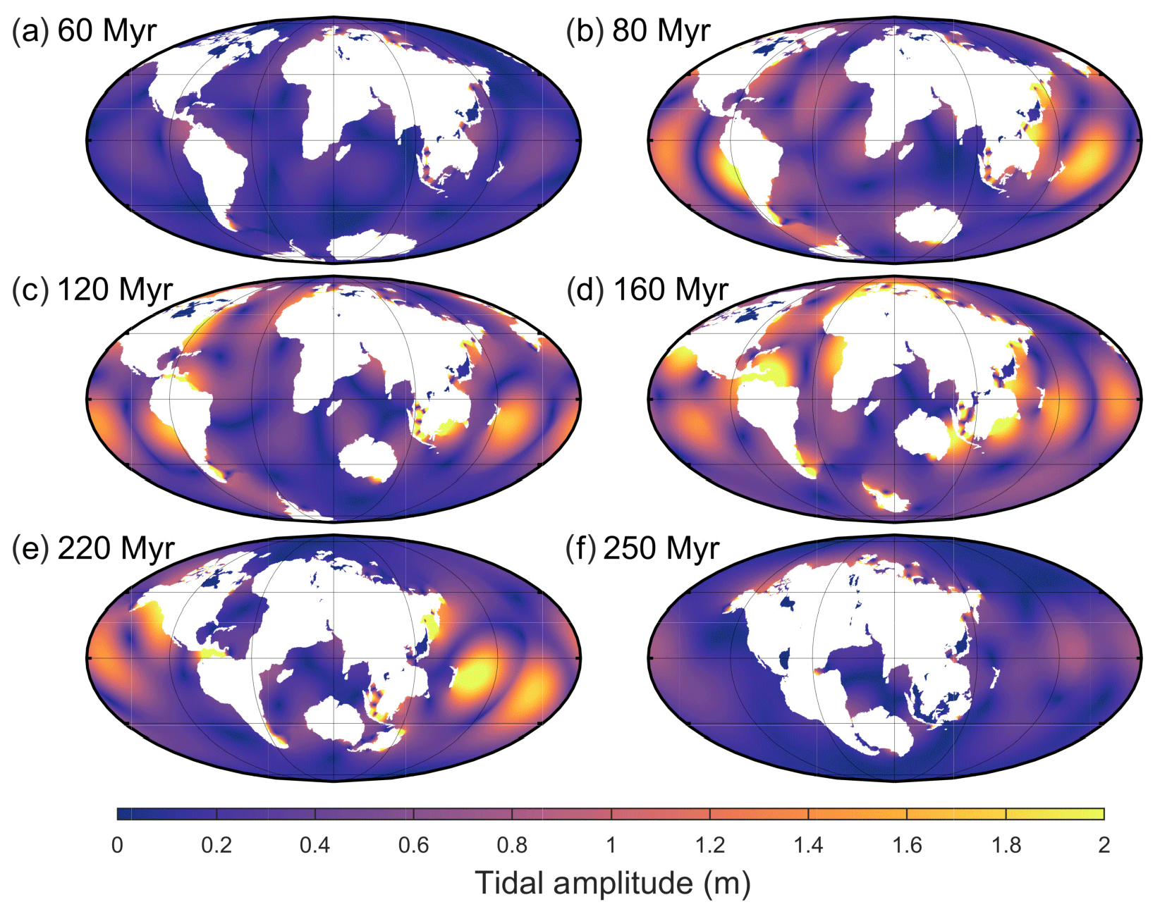
Figure 2Global M2 amplitudes for six representative time slices of the Pangaea Ultima scenario. The colour scale saturates at 2 m. For the full set of time slices covering every 20 Myr, see the Supplement. Additionally, note that the figures presented for each scenario display different time slices to highlight periods with interesting tidal signals and that the centre longitude varies between panels to ensure the supercontinent forms in the middle of each figure (where possible).
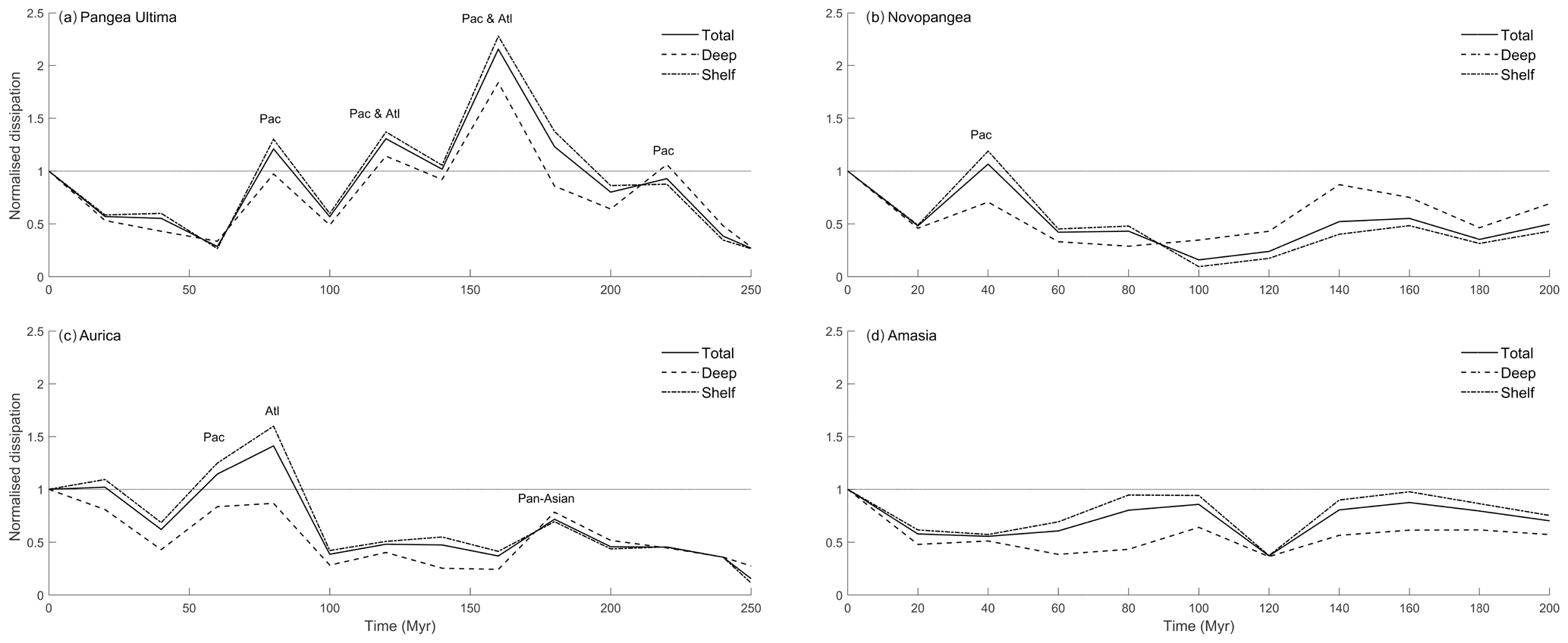
Figure 3Normalized (against PD degenerate) globally integrated dissipation rates for the Pangaea Ultima (a), Novopangaea (b), Aurica (c), and Amasia (d) scenarios. The lines refer to total (solid line), deep (dashed line), and shelf (dotted–dashed line) integrated dissipation values. Each super-tidal peak is marked where it reaches its peak. Pac stands for Pacific and Atl stands for Atlantic.
The resulting tidal amplitudes and associated integrated dissipation rates are shown in Figs. 2, 4–6 (amplitudes), and 3 (dissipation). The latter is split into the global total rate and rates in shallow (depths of < 500 m) and deep water (depths of > 500 m; Egbert and Ray, 2001) to highlight the mechanisms behind the energy loss. In the following we define a super-tide as occurring when (i) tidal amplitudes in a basin are on average meso-tidal or above, i.e. larger than 2 m, and (ii) the globally integrated dissipation is equivalent to or larger than present-day values.
3.1 Pangaea Ultima
In the Pangaea Ultima scenario, the Atlantic Ocean continues to open for another 100 Myr, after which it starts closing, leading to the formation of a slightly distorted new Pangaea in 250 Ma (Fig. 2 and Davies, 2019a). The continued opening of the Atlantic in the first 60 Myr moves the basin out of resonance, causing the M2 tidal amplitude and dissipation to gradually decrease (Figs. 2 and 3a). During this period, the total global dissipation drops to below 30 % of the PD (present-day) rate (note that this is equivalent to 2.2 TW, as we compare it to the degenerate bathymetry simulation), after which, at 80 Ma, it increases rapidly to 120 % of PD (Figs. 3a and 2b). This peak at 80 Ma is due to a resonance in the Pacific Ocean initiated by the shrinking width of the basin (Fig. 2b). The dissipation then drops again until it recovers and peaks around 120 Ma at 130 % above PD (Fig. 3a). This second peak is caused by another resonance in the Pacific, combined with a local resonance in the northwestern Atlantic (Fig. 2c). This period also marks the initiation of closure of the trans-Antarctic ocean, a short-lived ocean, which began opening at 40 Ma and was micro-tidal for its entire tenure (Fig. 2a–c). A third peak then occurs at 160 Ma, the most energetic period of the simulation, with the tides being 215 % more energetic than at present due to both the Atlantic and the Pacific being resonant for M2 frequencies (Fig. 2d). After this large-scale double resonance, the first described in detail in deep-time simulations and the most energetic relative dissipation rate encountered, the tidal energy drops, with a small recovery occurring at 220 Ma due to a further minor Pacific resonance (Fig. 2e). When Pangaea Ultima forms at 250 Ma (see Fig. 2f), the global energy dissipation has decreased to 25 % of the PD value or 0.5 TW (Fig. 2f).
3.2 Novopangaea
In the Novopangaea scenario, the Atlantic Ocean continues to open for the remainder of the supercontinent cycle. Consequently, the Pacific closes, leading to the formation of a new supercontinent at the antipodes of Pangaea in 200 Ma (Fig. 4 and Davies, 2019b). As a result, within the next 20 Myr the global M2 dissipation rates decrease to half of present-day values (see Figs. 3b and 4). The energy then recovers to PD levels at 40 Ma as a result of the Pacific Ocean becoming resonant. From 40 to 100 Myr, the dissipation rates drop, reaching 15 % of the PD value at 100 Ma. There is a subsequent recovery to values close to 50 % of PD, with a tidal maximum at 160 Ma due to local resonance in the newly formed East African Ocean (Davies et al., 2018). Even though the tidal amplitude in this new ocean reaches meso-tidal levels (i.e. 2–4 m tidal range, Fig. 3b), the increased dissipation in this ocean only increases the global total tidal dissipation to 50 % PD (Fig. 4e). Therefore, this ocean cannot be considered super-tidal. The tides then remain at values close to half of present day, i.e. equal to the long-term mean over the past 250 Myr in Green et al. (2017), until the formation of Novopangaea at 200 Ma. After 100 Myr there is a regime shift in the location of the dissipation rates, with a larger fraction dissipated in the deep ocean than before (Fig. 3b).
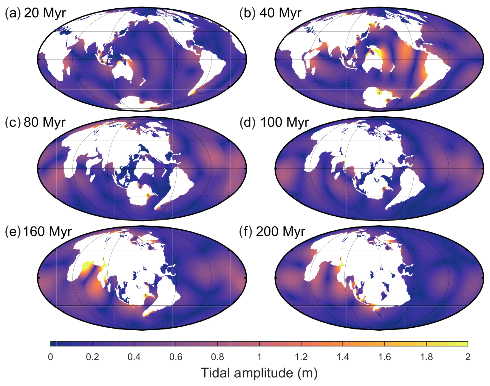
Figure 4The same as in Fig. 2 but for the Novopangaea scenario.
3.3 Aurica
Aurica is characterized by the simultaneous closing of both the Atlantic and the Pacific Oceans and the emergence of the new pan-Asian Ocean. This allows Aurica to form via combination in 250 Ma (Fig. 5 and Davies, 2019c). In this scenario, the tides remain close to present-day values for the next 20 Myr (see Figs. 3c and 5 for the results), after which they drop to 60 % of PD at 40 Ma, only to rise to 114 % of PD values at 60 Ma, and then to 140 % of PD rates at 80 Ma. This period hosts a relatively long super-tidal period, lasting at least 40 Myr, as the Pacific and Atlantic go in and out of resonances at 60 and 80 Ma, respectively. The dissipation then drops to 40 %–50 % of PD, with a local peak of 70 % of the PD value at 180 Ma due to resonance in the pan-Asian Ocean. This is the same age as the North Atlantic today, which strongly suggests that oceans go through resonance around this age. By the time Aurica forms, at 250 Ma, the dissipation is 15 % of PD, the lowest of all simulations presented here.
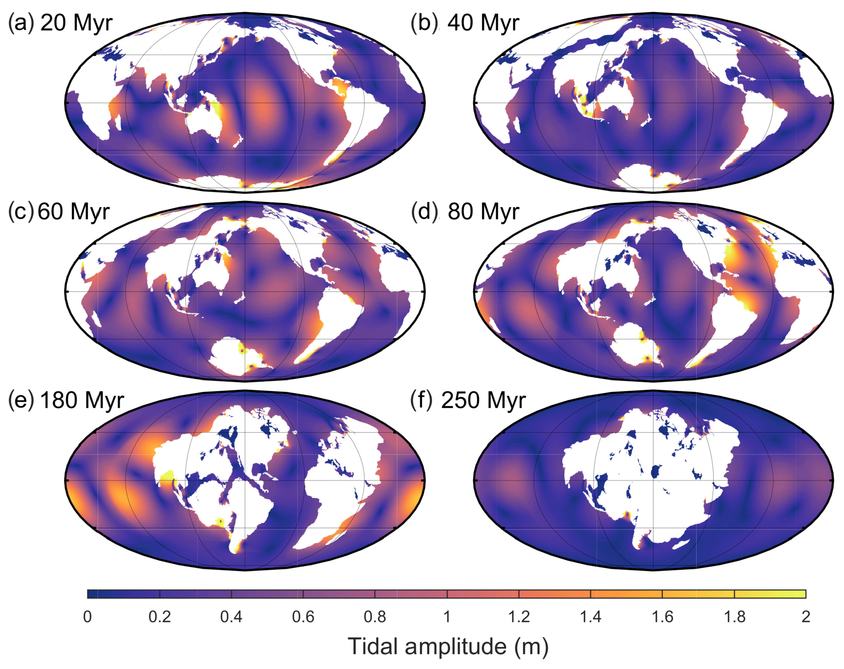
Figure 5The same as in Fig. 2 but for the Aurica scenario.
3.4 Amasia
In the Amasia scenario, all the continents except Antarctica move north, closing the Arctic Ocean and forming a supercontinent around the North Pole in 200 Ma (Fig. 6 and Davies, 2019d). The results show that the M2 tidal dissipation drops to 60 % of PD rates within the next 20 Myr (Figs. 3d and 6 for continued discussion). This minimum is followed by a consistent increase, reaching 80 % of PD rates at 100 Ma, and then, after another minimum of 40 % of PD rates at 120 Ma, tidal dissipation increases until it reaches a maximum of 85 % at 160 Ma. These two maxima are a consequence of several local resonances in the North Atlantic, North Pacific, and along the coast of South America, and the minimum at 120 Ma is a result of the loss of the dissipative Atlantic shelf areas due to continental collision. A major difference between Amasia and the scenarios previously described is that here we never encounter a full basin-scale resonance. This is because the circumpolar equatorial ocean that forms is too large to host tidal resonances and the closing Arctic Ocean is too small to ever become resonant. However, the scenario is still rather energetic, with dissipation rates averaging around 70 % of PD rates because of several local areas of high tidal amplitudes and corresponding high shelf dissipation rates (Fig. 3d).
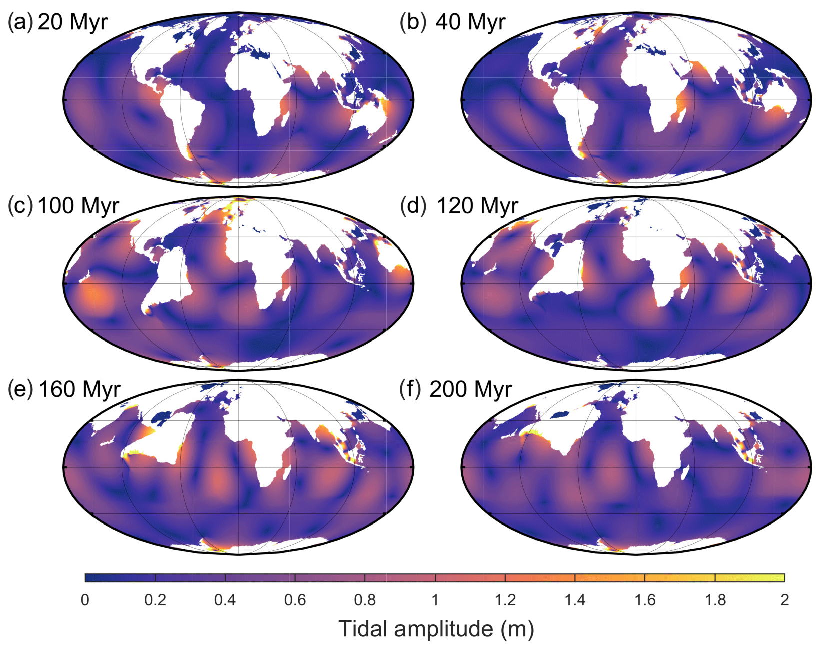
Figure 6The same as in Fig. 2 but for the Amasia scenario.
Table 1Summary of the number of super-tidal peaks for each scenario.

* Against PD degenerate =2.2 TW.
We investigated how the tides may evolve during four probable scenarios of the formation of Earth's future supercontinent. The results show large variations in tidal energetics between the scenarios (see Table 1 and Fig. 3), with the number of tidal maxima ranging from 1 (at present during the Amasia scenario) to 5 (including today's in the Pangaea Ultima scenario); see Table 1 for a summary. These maxima occur because of tidal resonances in the ocean basins as they open and close. Furthermore, we have shown that an ocean basin becomes resonant for the M2 tide when it is around 140–180 Myr old (as is the PD Atlantic). The reason for this is simple: assuming the net divergence rate of two continents bordering each side of an ocean basin is ∼3 cm yr−1 (which is close to the average drift rates today), after 140 Myr it will be 4500 km wide. Tidal resonance occurs when the basin width is half of the tidal wavelength (Arbic and Garrett, 2010):
where the wave speed is given by
and T is the tidal period (12.42 h). For a 4000 m deep ocean, resonance thus occurs when the ocean is 4429 km wide, i.e. at the age given above. The depth of the simulated oceans changes between the scenarios to preserve ocean volume at that of present day. These changes are too small to affect the resonant scales in the different simulations, especially at the resolution we are using here (0.25∘ in latitude and longitude). For example, in the Novopangaea scenario, which has the shallowest average ocean depth at 3860 m, the resonant basin scale is 4350 km, whereas in the Pangaea Ultima scenario, in the present day the overall deepest at 4395 m, the basin scale would be 4642 km. This again highlights the relationship between the tidal and tectonic evolution of an ocean basin. It also reiterates that ocean basins must open for at least 140 Myr to be resonant during their opening at present-day drift speeds (e.g. the pan-Asian ocean). If an ocean opens for less than 140 Myr, e.g. the trans-Antarctic (80 Myr of opening) or Arctic ocean (60 Myr of opening; Miller et al., 2006), or if they drift slower than 3 cm yr−1, they will not become resonant. After this 140 Myr and 4500 km age and width threshold has been reached, the ocean may then be resonant again if it closes.
Therefore, if the geometry and mode of supercontinent formation permits (i.e. multiple Wilson cycles are involved), several oceans may go through multiple resonances – sometimes simultaneously – as they open and close during a supercontinent cycle. For example, in the Pangaea Ultima scenario, the Atlantic and Pacific are simultaneously resonant at 160 Ma (Table 1), and, as Aurica forms, the Atlantic is resonant twice (at present and when closing at 80 Ma), the Pacific is resonant once (closing), and the pan-Asian ocean is resonant once (after 180 Ma, when opening; Table 1 and Sect. 3.3).
Table 2Summary of the total time each scenario was in a super-tidal state.
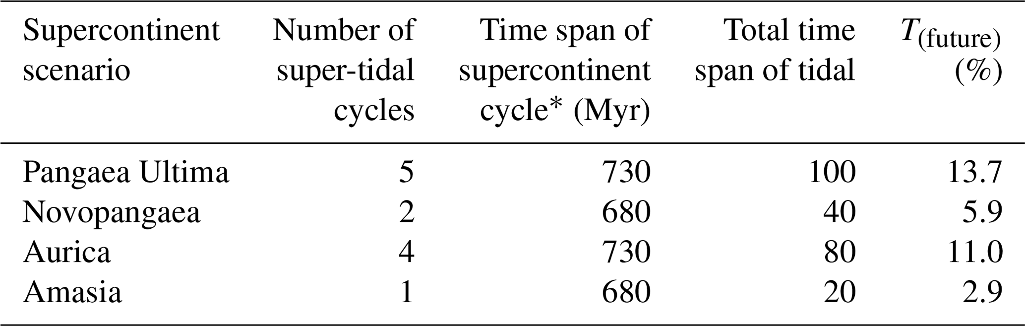
* From the formation of maxima (Myr) Pangaea to the break-up of the future supercontinent.
The simulations here expand on the work of Green et al. (2018) regarding the tidal evolution of Aurica. They find a more energetic future compared to the present Aurica simulations (e.g. our Fig. 3c): their average tidal dissipation is 84 % of the PD value, with a final state at 40 % of PD, whereas we find dissipation at 64 % of PD on average and 15 % of PD at 250 Myr. This discrepancy can be explained by two factors present in the work of Green et al. (2018): a lack of temporal resolution and a systematic northwards displacement in the configuration of the continents, meaning their tidal maxima are exaggerated. Despite these differences, the results are qualitatively similar, and we demonstrate here that under this future scenario the tides will be even less energetic than suggested in Green et al. (2018). This, along with results from tidal modelling of the deep past (Green et al., 2017, this paper, and unpublished results) lends further support to the super-tidal cycle concept and again shows how strong the current tidal state is.
All four scenarios presented have an average tidal dissipation lower than the present day, and all scenarios, except Amasia, have a series of super-tidal periods analogous to present day. The results presented here can supplement the fragmented tidal record of the deep past (Kagan and Sundermann, 1996; Green et al., 2017) and allow us to draw more detailed conclusions about the evolution of the tide over geological time, and the link between the tide, the supercontinent cycle, and the Wilson cycle.
We have estimated the number tidal maxima that have occurred in the Earth's history (N) and the total time that the Earth was in a super-tidal state (T) as follows:
and
Nsc represents the number of supercontinent cycles that have occurred on Earth, including the present one (we assume a minimum of five supercontinent cycles; e.g. Davies et al., 2018, and references therein), Nwc is the number of Wilson cycles per supercontinent cycle (we assume an average of two), Nt is the number of tidal maxima per Wilson cycle (we assume an average of two; this work). Ttm is a representative time duration for each tidal maximum (20 Myr), and TE is the age of the Earth (4.5 Gyr; e.g. Brent, 2001). This Fermi estimation suggests that there may have been ∼20 super-tidal periods on Earth (N) spanning over 400 Myr (8.9 %) of the Earth's history. This value is corroborated by the results in Table 2.
The data generated and used in the current study are available in the OSF (Open Science Framework) repository and can be accessed at https://doi.org/10.17605/OSF.IO/8NEQ4 (Davies, 2020). The data is freely available to use according to the CC0 1.0 license.
The figures available in the supplement have been made into four short videos illustrating the tidal evolution (in 20 Myr increments) of each scenario as they progress from the present day to the eventual formation of the next supercontinent. The Pangea Ultima scenario is illustrated in video S1 (Davies, 2019a, https://doi.org/10.5446/43738). The Novopangea scenario is illustrated in video S2 (Davies, 2019, https://doi.org/10.5446/43739). The Aurica scenario is illustrated in video S3 (Davies, 2019, https://doi.org/10.5446/43740). The Amasia scenario is illustrated in video S4 (Davies, 2019, https://doi.org/10.5446/43741).
The supplement related to this article is available online at: https://doi.org/10.5194/esd-11-291-2020-supplement.
HSD contributed to conceptualization, formal analysis, investigation, methodology, software, validation, visualization, writing of the original draft, and the review and editing process.
JAMG contributed to conceptualization, data curation, funding acquisition, methodology, project administration, resources, software, supervision, validation, and the review and editing process.
JCD contributed to conceptualization, funding acquisition, project administration, resources, supervision, and the review and editing process.
The authors declare that they have no conflict of interest.
Hannah S. Davies acknowledges funding from FCT (ref. UIDB/50019/2020 – Instituto Dom Luiz; FCT PhD grant ref. PD/BD/135068/2017). J. A. Mattias Green acknowledges funding from NERC (MATCH, NE/S009566/1), an internal travel grant from the School of Ocean Science, and a Santander travel bursary awarded through Bangor University. Joao C. Duarte acknowledges an FCT Researcher contract, an exploratory project grant (ref. IF/00702/2015), and the FCT project UIDB/50019/2020 – Instituto Dom Luiz. Tidal modelling was carried out using HPCWales with the support of Ade Fewings. We would like to thank Filipe Rosas, Pedro Miranda, Wouter Schellart, and Célia Lee for their insightful discussions and for providing support related to several aspects of the work. We would also like to thank Daniel Pastor-Galán, the anonymous reviewer, and the editor Ira Didenkulova for their efforts in providing constructive comments and moderation, which we believe have improved the paper.
This research has been supported by the Fundação para a Ciência e a Tecnologia through grant no. UIDB/50019/2020 – Instituto Dom Luiz, grant no. IF/00702/2015, and PhD grant no. PD/BD/135068/2017 and the Natural Environment Research Council (grant no. NE/S009566/1).
This paper was edited by Ira Didenkulova and reviewed by Daniel Pastor-Galán and one anonymous referee.
Amante, C. and Eakins, B. W.: ETOPO1 1 Arc-Minute Global Relief Model: Procedures, Data Sources and Analysis. NOAA Technical Memorandum NESDIS NGDC-24, National Geophysical Data Center, NOAA, https://doi.org/10.7289/V5C8276M, 2009.
Arbic, B. K. and Garrett, C.: A coupled oscillator model of shelf and ocean tides, Cont. Shelf Res., 30, 564–574, https://doi.org/10.1016/j.csr.2009.07.008, 2010.
Bradley, D. C.: Secular trends in the geologic record and the supercontinent cycle, Earth-Sci. Rev., 108, 16–33, https://doi.org/10.1016/j.earscirev.2011.05.003, 2011.
Brent, D. G.: The age of the Earth in the twentieth century: a problem (mostly) solved, Geol. Soc. Sp., 190, 1–14, https://doi.org/10.1144/GSL.SP.2001.190.01.14, 2001.
Burke, K.: Plate Tectonics, the Wilson Cycle, and Mantle Plumes: Geodynamics from the Top, Annu. Rev. Earth Pl. Sci., 39, 1–29, https://doi.org/10.1146/annurev-earth-040809-152521, 2011.
Conrad, C. P. and Lithgow-Bertelloni, C.: How Mantle Slabs Drive Plate Tectonics, Science, 298, 207–209, https://doi.org/10.1126/science.1074161, 2002.
Davies, H.: Pangea Ultima M2 tidal amplitude in 20 myr increments, https://doi.org/10.5446/43738, 2019a.
Davies, H.: Novopangea M2 tidal amplitudes in 20 myr increments, https://doi.org/10.5446/43739, 2019b.
Davies, H.: Aurica M2 tidal amplitudes in 20 myr increments, https://doi.org/10.5446/43740, 2019c.
Davies, H.: Amasia M2 tidal amplitudes in 20 myr increments, https://doi.org/10.5446/43741, 2019d.
Davies, H.: Back to the future II: Tidal evolution of four supercontinent scenarios, https://doi.org/10.17605/OSF.IO/8NEQ4, 2020.
Davies, H. S., Green, J. A. M., and Duarte, J. C.: Back to the future: Testing different scenarios for the next supercontinent gathering, Global Planet. Change, 169, 133–144, https://doi.org/10.1016/j.gloplacha.2018.07.015, 2018.
Duarte, J. C., Schellart, W. P., and Rosas, F. M.: The future of Earth's oceans: consequences of subduction initiation in the Atlantic and implications for supercontinent formation, Geol. Mag., 155, 45–58, https://doi.org/10.1017/S0016756816000716, 2018.
Egbert, G. D. and Erofeeva, S. Y.: Efficient Inverse Modeling of Barotropic Ocean Tides, J. Atmos. Ocean. Tech., 19, 183–204, 2002.
Egbert, G. D. and Ray, R. D.: Estimates of M2 tidal energy dissipation from Topex/Poseidon altimeter data, J. Geophys. Res., 106, 22475–22502, https://doi.org/10.1029/2000JC000699, 2001.
Egbert, G. D., Ray, R. D., and Bills, B. G.: Numerical modelling of the global semidiurnal tide in the present day and in the last glacial maximum, J. Geophys. Res., 109, C03003, https://doi.org/10.1029/2003JC001973, 2004.
Golonka, J.: Late Triassic and Early Jurassic palaeogeography of the world, Palaeogeogr. Palaeocl., 244, 297–307, https://doi.org/10.1016/j.palaeo.2006.06.041, 2007.
Green, J. A. M.: Ocean tides and resonance, Ocean Dynam., 60, 1243–1253, https://doi.org/10.1007/s10236-010-0331-1, 2010.
Green, J. A. M. and Huber, M.: Tidal dissipation in the early Eocene and implications for ocean mixing, Geophys. Res. Lett., 40, 2707–2713, https://doi.org/10.1002/grl.50510, 2013.
Green, J. A. M., Huber, M., Waltham, D., Buzan, J., and Wells, M.: Explicitly modelled deep-time tidal dissipation and its implication for Lunar history, Earth Planet. Sc. Lett., 461, 46–53, https://doi.org/10.1002/2017gl076695, 2017.
Green, J. A. M., Molloy, J. L., Davies, H. S., and Duarte, J. C.: Is There a Tectonically Driven Supertidal Cycle?, Geophys. Res. Lett., 45, 3568–3576, https://doi.org/10.1002/2017gl076695, 2018.
Hatton, C. J.: The superocean cycle, S. Afr. J. Geol., 100, 301–310, 1997.
Kagan, B. A.: Earth-Moon tidal evolution: model results and observational evidence, Prog. Oceanogr., 40, 109–124, https://doi.org/10.1016/S0079-6611(97)00027-X, 1997.
Kagan, B. A. and Sundermann, J.: Dissipation of Tidal energy, Paleotides and evolution of the Earth-Moon system, Adv. Geophys., 38, 179–266, https://doi.org/10.1016/S0065-2687(08)60021-7, 1996.
Miller, E. L., Toro, J., Gehrels, G., Amato, J. M., Prokopiev, A., Tuchkova, M. I., Akinin, V. V., Dumitru, T. A., Moore, T. E., and Cecile, M. P.: New insights into Arctic paleogeography and tectonics from U-Pb detrital zircon geochronology, Tectonics, 25, TC3013, https://doi.org/10.1029/2005TC001830, 2006.
Mitchell, R. N., Kilian, T. M., and Evans, D. A. D.: Supercontinent cycles and the calculation of absolute palaeolongitude in deep time, Nature, 482 208–211, https://doi.org/10.1038/nature10800, 2012.
Müller, R. D., Cannon, J., Qin, X., Watson, R. J., Gurnis, M., Williams, S., Pfaffelmoser, T., Seton, M., Russell, S. H. J., and Zahirovic, S.: GPlates – Building a Virtual Earth Through Deep time, Geochem. Geophy. Geosy., 19, 2243–2261, https://doi.org/10.1029/2018GC007584, 2018.
Murphy, J. B. and Nance, R. D.: Do supercontinents introvert of extrovert?: Sm-Nd isotope evidence, Geol. Soc. Am., 31, 873–876, https://doi.org/10.1130/G19668.1, 2003.
Murphy, J. B. and Nance, R. D.: Do Supercontinents turn inside-in or inside-out?, Int. Geol. Rev., 47, 591–619, https://doi.org/10.2747/0020-6814.47.6.591, 2005.
Murphy, J. B. and Nance, R. D.: The Pangea conundrum, Geol. Soc. Am., 36, 703–706, https://doi.org/10.1130/G24966A.1, 2008.
Nance, D. R., Worsley, T. R., and Moody, J. B.: The Supercontinent Cycle, Sci. Am., 259, 72–78, https://doi.org/10.1038/scientificamerican0788-72, 1988.
Nance, D. R., Murphy, B. J., and Santosh, M.: The supercontinent cycle: A retrospective essay, Gondwana Res., 25, 4–29, https://doi.org/10.1016/j.gr.2012.12.026, 2013.
Nield, T.: Supercontinent, Granta Books, London, 287 pp., 2007.
Pastor-Galan, D., Nance, D. R., Murphy, B. J., and Spencer, C. J.: Supercontinents: myths, mysteries, and milestones, Geological Soc. London, 470, 39–64, https://doi.org/10.1144/SP470.16, 2018.
Platzmann G. W.: Normal modes of the Atlantic and Indian oceans, J. Phys. Oceanogr., 5, 201–221, 1975.
Qin, X., Müller, R. D., Cannon, J., Landgrebe, T. C. W., Heine, C., Watson, R. J., and Turner, M.: The GPlates Geological Information Model and Markup Language, Geosci. Instrum. Method. Data Syst., 1, 111–134, https://doi.org/10.5194/gi-1-111-2012, 2012.
Scotese, C. R.: Jurassic and cretaceous plate tectonic reconstructions, Palaeogeogr. Palaeocl., 87, 493–501, https://doi.org/10.1016/0031-0182(91)90145-H, 1991.
Scotese, C. R.: Palaeomap project, available at: http://www.scotese.com/earth.htm (last access: 15 January 18), 2003.
Smith, W. H. F. and Sandwell, D. T.: Global seafloor topography from satellite altimetry and ship depth soundings, Science, 277, 1956–1962, https://doi.org/10.1126/science.277.5334.1956, 1997.
Stammer, D., Ray, R. D., Andersen, O. B., Arbic, B. K., Bosch, W., Carrère, L., Cheng, Y., Chinn, D. S., Dushaw, B. D., Egbert, G. D., Erofeeva, S. Y., Fok, H. S., Green, J. A. M., Griffiths, S., King, M. A., Lapin, V., Lemoine, F. G., Luthcke, S. B., Lyard, F. Morison, J., Müller, M., Padman, L., Richman, J. G., Shriver, J. F., Shum, C. K., Taguchi, E., and Yi, Y.: Accuracy assessment of global barotropic ocean tide models, Rev. Geophys., 52, 243–282, https://doi.org/10.1002/2014RG000450, 2014.
Torsvik, T. H., Burke, K., Steinberger, B., Webb, S. J., and Ashwal, L. D.: Diamonds sampled by plumes from the core-mantle boundary, Nature, 466, 352–357, https://doi.org/10.1038/nature09216, 2010.
Torsvik, T. H., Steinberger, B., Ashwal, L. D., Doubrovine, P. V., and Trønnes, R. G.: Earth evolution and dynamics – a tribute to Kevin Burke, Can. J. Earth Sci., 53, 1073–1087, https://doi.org/10.1139/cjes-2015-0228, 2016.
Wilmes, S. B. and Green, J. A. M.: The evolution of tides and tidal dissipation over the past 21,000 years, J. Geophys. Res.-Ocean, 119, 4038–4100, https://doi.org/10.1002/2013JC009605, 2014.
Wilson, T. J.: Did the Atlantic Close and then Re-Open?, Nature, 211, 676–681, https://doi.org/10.1038/211676a0, 1966.
Yoshida, M.: Formation of a future supercontinent through plate motion – driven flow coupled with mantle downwelling flow, Geol. Soc. Am., 44, 755–758, https://doi.org/10.1130/G38025.1, 2016.
Yoshida, M. and Santosh, M.: Future supercontinent assembled in the northern hemisphere, Terra Nova, 23, 333–338, https://doi.org/10.1111/j.1365-3121.2011.01018.x, 2011.
Yoshida, M. and Santosh, M.: Geoscience Frontiers voyage of the Indian subcontinent since Pangea breakup and driving force of supercontinent cycles: insights on dynamics from numerical modelling, Geosci. Front., 9, 1–14, https://doi.org/10.1016/j.gsf.2017.09.001, 2017.
Yoshida, M. and Santosh, M.: Voyage of the Indian subcontinent since Pangea breakup and driving force of supercontinent cycles: Insights on dynamics from numerical modelling, Geosci. Front., 9, 1279–1292, https://doi.org/10.1016/j.gsf.2017.09.001, 2018.
Zaron, E. D. and Egbert, G. D.: Verification studies for a z-coordinate primitive-equation model: Tidal conversion at a mid-ocean ridge, Ocean Model., 14, 257–278, https://doi.org/10.1016/j.ocemod.2006.05.007, 2006.