2.1 Data

For our study we use the meteorological fields of the CESM-LE produced by the fully coupled CESM1 used in CMIP5 (Kay et al., 2015). Between 1920 and 2005 the CESM-LE simulations follow the CMIP5 historical experimental design (Taylor et al., 2012; Lamarque et al., 2010), while after 2005 to 2100 they follow the RCP8.5 scenario (Van Vuuren et al., 2011). In the study we utilize sea surface temperature (SST) and total precipitation (PRECT) fields with a horizontal resolution of 1^∘ × 1^∘ and 1.25^∘ × 0.942^∘, respectively. Due to the small systematic difference between the members run at the National Center for Atmospheric Research (NCAR) and at the Toronto supercomputer (CESM-LE, 2016) we utilize only the members from the NCAR simulations. Taking into consideration the convergence time of the simulations, we only deal with data from 1950 onward.

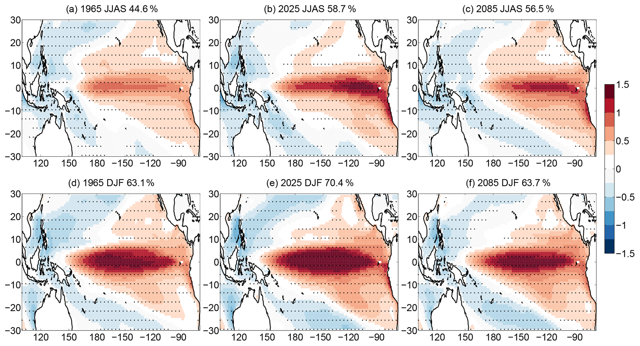
Figure 1Ensemble-based SST regression maps [in degrees Celsius] for years given in the title of the panel for (a–c) JJAS and (d–f) DJF. The explained variance in the first SEOF mode is also displayed in the title of the panels. Dots represent geographical locations where the regression coefficient is significant at the 95 % level. For better visibility, only every fourth grid point is dotted.

2.2 Studying ENSO and its teleconnections in the snapshot framework

Here, we study ENSO by evaluating the variability in the SST field over the ensemble members at each time instant in the Pacific using the SEOF method. It is based on the region of (30^∘ S, 30^∘ N) × (100^∘ E, 70^∘ W), which is also chosen in Maher et al. (2018) for their EOF-E analysis. To eliminate the distorting impact of the regular latitude–longitude grid in the EOF analysis, the SST fields are weighted by the square root of the cosine of the latitude, following Thompson and Wallace (2000). We consider the instantaneous ensemble-based leading SEOF mode (by which we mean the normalized eigenvectors associated with the largest eigenvalue of the covariance matrix of the SST anomaly fields) as the ENSO loading pattern and the phase of the phenomenon in each member as the corresponding principal component (PC1). With the sign of the SEOF patterns which shall be used in Fig. 1, PC1 > 0 (PC1 < 0) corresponds to anomalously warm (cold) events associated with above (below) the ensemble average SST in the central and east-central equatorial Pacific Ocean. As in Thompson and Wallace (2000), not the normalized EOF patterns, but rather the SST regression maps are shown, computed by regressing the unweighted SST anomaly fields onto the standardized PC1 data. Therefore, the values appearing on the regression maps characterize typical amplitudes in the variability in the SST. The instantaneous strength of ENSO is computed as the ensemble standard deviation of the PC1s of the given time instant, as the snapshot counterpart of the temporal standard deviation of the PC1, used as a common practice to represent the strength of an oscillation in traditional EOF analysis (Monahan and Dai, 2004; Maher et al., 2018). For comparison, we also analyze the time evolution of the ensemble-based ENSO Niño3 amplitude defined by the ensemble standard deviation of Niño3 index in the (5^∘ S, 5^∘ N) × (150, 90^∘ W) Niño3 region.

Note that PC1 is actually an index for the ENSO phase. It is found to be closely related to the standard Niño3 index, with a correlation coefficient of 0.98 (Ashok et al., 2007), which confirms that the first mode of EOF represents the conventional ENSO well. It has been used in this way in other studies as well; see, e.g., Diaz et al. (2001) who carried out traditional EOF analysis using a slightly smaller Pacific region. As an index, its main use is a standardized indication for the state of the remote phenomena related to ENSO. Even though more complex indices exist nowadays for the characterization of ENSO, created, e.g., by the combination of PC1 and PC2, such as the ones in Takahashi et al. (2011), we choose PC1 to provide a simple and easy-to-follow example, illustrating the applicability and advantages of the SEOF analysis.

For characterizing such teleconnections, an instantaneous ensemble-based correlation coefficient can be determined between the PC1 and PRECT data of the ensemble members at each time instant and for each grid point. As ENSO has its maximum around boreal winter, which is traditionally defined as DJF, we analyze the DJF ENSO pattern and ENSO teleconnections in the paper. In order to investigate the possibility of predicting precipitation half a year in advance based on PC1, we calculate lagged correlations beyond instantaneous ones. The relationship between ENSO and the South Asian monsoon is believed to be one of the most important teleconnection phenomena and is traditionally investigated using JJAS (see, e.g., Krishna Kumar et al., 1999; Ashok et al., 2007; Srivastava et al., 2019), and western Africa also receives the major proportion of its annual rainfall in JJAS (Srivastava et al., 2019); therefore, we utilize both DJF-mean and JJAS-mean data in order to reveal simultaneous and lagged connections and to correlate the JJAS PC1 with the JJAS PRECT, the DJF PC1 with the DJF PRECT, the DJF PC1 with the JJAS PRECT, and the JJAS PC1 with the DJF PRECT over the ensemble. The choice of DJF and JJAS seasons is also used in Wu et al. (2012) for studying the ENSO influences on Indian summer monsoon. The investigation of lagged correlations opens up the possibility of studying the predictability of the amount of precipitation in different regions based on the PC1.

2.3 Comparing the capabilities of the snapshot and traditional methods

To better understand the facilities of the snapshot methods in general, it is worth giving an overview of the advantages and limitations of both the snapshot methods and traditional temporal ones. When only single time series are available, such as measurements or single time series of model simulations, one has to use the traditional temporal methods of time series analysis to investigate a phenomenon. For example, in the case of ENSO, when examining its characteristics by EOF analysis, used in this study as well, it means that for the time period of the analysis a single EOF loading pattern is obtained, i.e., the spatial pattern of the oscillation must be assumed to be constant for the given time period. The phases of this “standing” oscillation over time are then provided by the corresponding PC1s, and the strength of ENSO teleconnections in the studied time period can be characterized at every geographical location by a single correlation coefficient between the PC1 time series and the local time series of the studied quantity. However, during this time period (e.g., within 30 or 100 years) climate changes (excluding the nonrealistic case of stationary forcing). For example, in the case of the CESM-LE climate change indeed manifests in a considerable global surface temperature increase on a decadal timescale between 1950 and 2100 (Kay et al., 2015). Therefore, it can be neither presupposed that the pattern of the ENSO or the strength of its teleconnections remain constant during climate change nor assumed that a single oscillation pattern or correlation coefficient can faithfully characterize the conditions of several years.

A changing climate may manifest even in local regime shifts and appearance of tipping cascades in such a coupled system (Klose et al., 2019). For a demonstration of the possibility of such cascading events in the climate system in a conceptual model of a coupled North Atlantic Ocean–ENSO system, see Dekker et al. (2018). These transitions may cause qualitative changes also in local dynamics and in the connections of the climate system. Climate change can also result in chaotic synchronization between certain regions which behave as chaotic oscillators (Duane, 1997), e.g., implying a change in the relationship between the Atlantic and Pacific sectors (Duane and Tribbia, 2001). As another example, Falasca et al. (2019) showed both in the CESM-LE and in reanalysis data that the connection between the equatorial Atlantic region and the ENSO may exist only in certain decades, possibly because of chaotic synchronization.

Naturally, the analyzed time period can be divided into smaller time windows, and then some kind of time-dependence of the oscillation and teleconnections can be studied. However, if the forcing is nonstationary, the climate can change even within shorter time periods. The smaller the time window, the less the climate is expected to change but meanwhile, the less robust the calculated statistics will be due to the smaller number of temporal data points. Regarding the case of changing climate, the optimal choice would obviously be to choose a series of time windows of length of one data point, within which the climate evidently cannot change. This is exactly what the snapshot methods do by calculating statistics at single time instants; however, an ensemble is needed for this purpose. Therefore, the methods of the snapshot framework operate across the ensemble dimension of climate realizations at single time instants and provide measures and statistics that characterize only the instantaneous potential states of the climate system without a direct impact of previous or future climate states on the value of the statistics, in contrast to results from traditional time series analysis operating along the time dimension. For example, the most known ensemble statistics, the ensemble mean and ensemble standard deviation, describe the mean state and the strength of the internal variability in the possibilities permitted by the instantaneous climate, respectively, at the chosen time instant under the external forcing history up to that time. Analogously, an instantaneous ensemble-based SEOF loading pattern represents the spatial structure of an oscillation that characterizes the potential variability in the climate states of the given time instant, and the corresponding PC1s reveal the phases in which the ensemble members are in that very moment.

A similar overview, comparing the results derived from snapshot methods and time series analysis, can be found in Herein et al. (2017) and Bódai et al. (2020) for the example of the North Atlantic Oscillation teleconnections using a station-based NAO index and the ENSO phenomenon using the Niño3 and Southern Oscillation (SOI) indices, respectively. The single time series results were shown to strongly differ from the snapshot ones. These papers also illustrate by numerical examples that the choice of the time window may have a considerable effect on the statistical measures in the traditional approach, while this is not a problem when using the snapshot framework.

As an obvious limitation, to take advantage of the methods within the snapshot framework to provide a mathematically correct way to describe the instantaneous statistics and characteristics of the potential climate states under the external forcing history up to that time, an ensemble of climate realizations is needed. The more reliable and robust the statistics aimed to be obtained are, the larger the required ensembles are. Note that the number of temporal data points is also an issue in the traditional time series analysis as well. We also feel important to repeat here that the desirable tools of a traditional time series analysis give robust and unbiased results only if the underlying statistics can be approximated well as stationary. Furthermore, temporal autocorrelation may seriously reduce the effective sample size of the traditional methodology; with a 3-year autocorrelation, the effective length of a 150-year time series is practically less than 50 data points.

Most often, an ensemble is produced by a climate model; however, they may also be accessible in experiments. For example, they proved to be useful in laboratory experiments aiming to study the effect of climate change on midlatitude atmospheric circulation (Vincze et al., 2017). Obviously, the obtained results are constrained by the climate model or the capability of the experimental setup, while the tools of time series analysis can be applied also to historical measurements or reanalysis data, i.e., for cases when only single time series exist due to the fact of having only one Earth history.

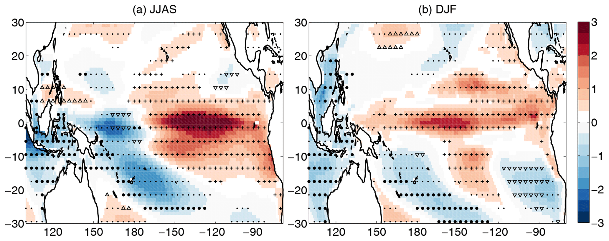
Figure 2The slope of the linear fit (10^−3 ∘C yr⁻¹) at each grid point of the (a) JJAS and (b) DJF regression maps from 1950 to 2100. Dots represent geographical locations where the trend is significant at the 95 % level. In addition, (i) where the trend is positive and the regression coefficients are positive and significant at the 95 % level in the temporal mean, “+” signs are displayed, (ii) where the trend is positive and the regression coefficients are negative and significant at the 95 % level in the temporal mean, “△” signs are displayed, (iii) where the trend is negative and the regression coefficients are positive and significant at the 95 % level in the temporal mean, “▿” signs are displayed, and (iv) where the trend is negative and the regression coefficients are negative and significant at the 95 % level in the temporal mean, “•” signs are displayed, respectively. For better visibility, the significance and direction of the trend is indicated at only every fourth grid point.

3.1 Changes in the ENSO pattern and amplitude

For a first impression of the SEOF analysis, the instantaneous ensemble-based regression maps of the first SEOF mode for the SST in the Pacific region for the JJAS period and DJF period are shown in Fig. 1a–c and d–f, respectively. As expected from observation-based data (see, e.g., Kirtman and Shukla, 2000), the typical amplitudes of the SST anomaly values across the ensemble members at the equatorial Pacific are somewhat larger in DJF than in JJAS. The shape of the pattern clearly changes somewhat over time, and the explained variance in the first SEOF mode also varies.

To determine whether the observed alterations are due to fluctuations because of the finite number of ensemble members or the consequences of the changing climate, a linear fit over time is performed on the ensemble-based regression maps at each grid point from 1950 to 2100 (Fig. 2). The applicability of linear fit to the time series of regression coefficients is checked at two random grid points in the region of strong positive trends and two other grid points in the region of negative trends in Fig. 2 for both seasons (see Fig. S1 in the Supplement), and the trend of the curves is found to be well approximated by linear regression. In the regression maps for JJAS (Fig. 2a) a positive trend with (1–3)$\times {\mathrm{10}}^{-\mathrm{3}}$ ^∘C yr⁻¹ can be detected in the Niño3 and Niño3.4 region, while close to Indonesia and Australia a clear negative trend with the same magnitude appears. It corresponds to an increase of 0.15 to 0.45 ^∘C in the SST variability, in 150 years (from 1950 to 2100), which is a considerable change compared to the magnitude of 0.1–1 ^∘C in the SST variability in Fig. 1. For DJF (Fig. 2b) a somewhat narrower band with slightly weaker increase of (0.5–2)$\times {\mathrm{10}}^{-\mathrm{3}}$ ^∘C yr⁻¹ can be seen all along the Equator in the Pacific Ocean and negative trends of a similar magnitude appear near Australia and at the western coast of South America. Similar trends in the annual ENSO pattern were pointed out in Maher et al. (2018) by EOF-E analysis mentioned in the Introduction, however, Fig. 2 draws attention to the fact that these patterns also have seasonal dependence. Ensemble-based instantaneous regression maps present typical values of the amplitude of the fluctuations directly related to the given EOF mode of variability at each grid point, which in the case of EOF1 has the strongest relationship with ENSO. The temporal changes in the regression maps are then easy to interpret intuitively; they show the changes in the fluctuation amplitudes, i.e., changes in the typical SST anomalies bound to the given mode at each grid point and potential shifting in the pattern during climate change as well. Nevertheless, it is also worth studying another representation of the ENSO pattern, namely the pattern which is separated from the amplitude of the phenomenon. The time series of this separated pattern, represented by the loading pattern of the SEOF analysis, and the changes in them are shown in Figs. S3 and S4, respectively. The temporal changes in these normalized patterns show the alterations in the relative importance of different regions from the point of view of the given mode. Their patterns in Fig. S4 are similar to the ones in Fig. 2; however, in contrast to them, no dominant maximum can be seen in the Niño3 region for DJF. Furthermore, while the amplitude increase in the Niño3 region in Fig. 2a in JJAS proves to be more pronounced than the decrease in the western part of the equatorial Pacific, Fig. S4 shows that the reduction of the relative importance of the latter is greater than the former one.

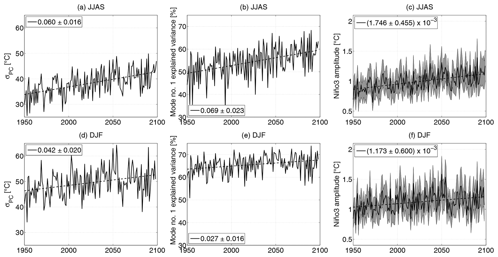
Figure 3(a, d) Ensemble-based ENSO strength as the ensemble standard deviation of the PC1 (σ_PC), (b, e) the explained variance in the first SEOF mode, and (c, f) Niño3 amplitude as the area-mean (thick line) ensemble standard deviation of SST in the Niño3 region and its area standard deviation (grey band) in (a–c) JJAS and (d–f) DJF. Linear fits are indicated by dashed lines; legends indicate the slope of the linear fits with 95 % confidence intervals.

Download

Another particularly important feature of the ENSO phenomenon is the ENSO amplitude, which shows a large diversity in different climate projections (Yeh and Kirtman, 2007; Collins et al., 2010; Chen et al., 2015). Therefore, besides the exploration of the changes in the ENSO pattern, we also quantify the potential changes in the ensemble-based instantaneous ENSO strength (the ensemble standard deviation of the PC1, σ_PC), and the change in the explained variance in the first SEOF mode (Fig. 3a, d, and b, e). Furthermore, the ensemble-based analog of a traditional amplitude of the ENSO phenomenon, namely the Niño3 amplitude, is also studied (Fig. 3c and f). The value of σ_PC is much smaller in JJAS (Fig. 3a) than in DJF (Fig. 3d), and Fig. 3b and d also show that the explained variance in the SST variability by the first SEOF mode is about 15 % greater in DJF than in JJAS. A systematic increase is found in all three quantities both for JJAS and DJF. The increase in JJAS is around 20 % for the σ_PC (Fig. 3a), the explained variance (Fig. 3b), as well as the ENSO amplitude (Fig. 3c), while the increase in DJF is somewhat lower, approximately 5 %–15 % for the three quantities. The larger values of the explained variance mean that by 2100 the oscillation associated with the first mode is going to be responsible for a much larger fraction of the variability in the SST fields. The increasing values in the explained variance in the first SEOF mode are found to be compensated for by the generally slightly decreasing trends appearing in the explained variance in higher-order modes (see Fig. S2). In JJAS, the second mode contributes the most to the decrease by 2.4 %, while in DJF, for which Fig. 3e shows a less pronounced increase for the first mode, the explained variance in the second mode is approximately constant, and the compensating decrease appears in the explained variance in the higher-order modes. For more details, see Fig. S2. The approximately 20 % increase in the Niño3 amplitude is in fairly good agreement with the study of Maher et al. (2018). It is comparable with the approximately 10 % increase within 100 years in Zheng et al. (2018) that was found for the CESM-LE for the Representative Concentration Pathway scenario with radiative forcing value of 8.5 W m⁻² in the year 2100 (RCP8.5) using sliding windows temporal statistics. This result reveals that the forced response of the ENSO amplitude under climate change is positive. Obviously this finding is valid for the CESM-LE only, while other models may behave differently regarding the ENSO amplitude (Yeh and Kirtman, 2007; Kim et al., 2014; Chen et al., 2015). We mention that the first ensemble-based study (which investigated several large ensembles) reported that an increase or zero trend is likely regarding the Niño3 amplitude change (Maher et al., 2018).

3.2 Changes in ENSO's teleconnections

To study the potential changes in the ENSO-related precipitation events over time, instantaneous ensemble-based correlation coefficients (r) between the PC1 and the total precipitation PRECT at each grid point are determined for both zero-lag and half-year-lagged PRECT data.

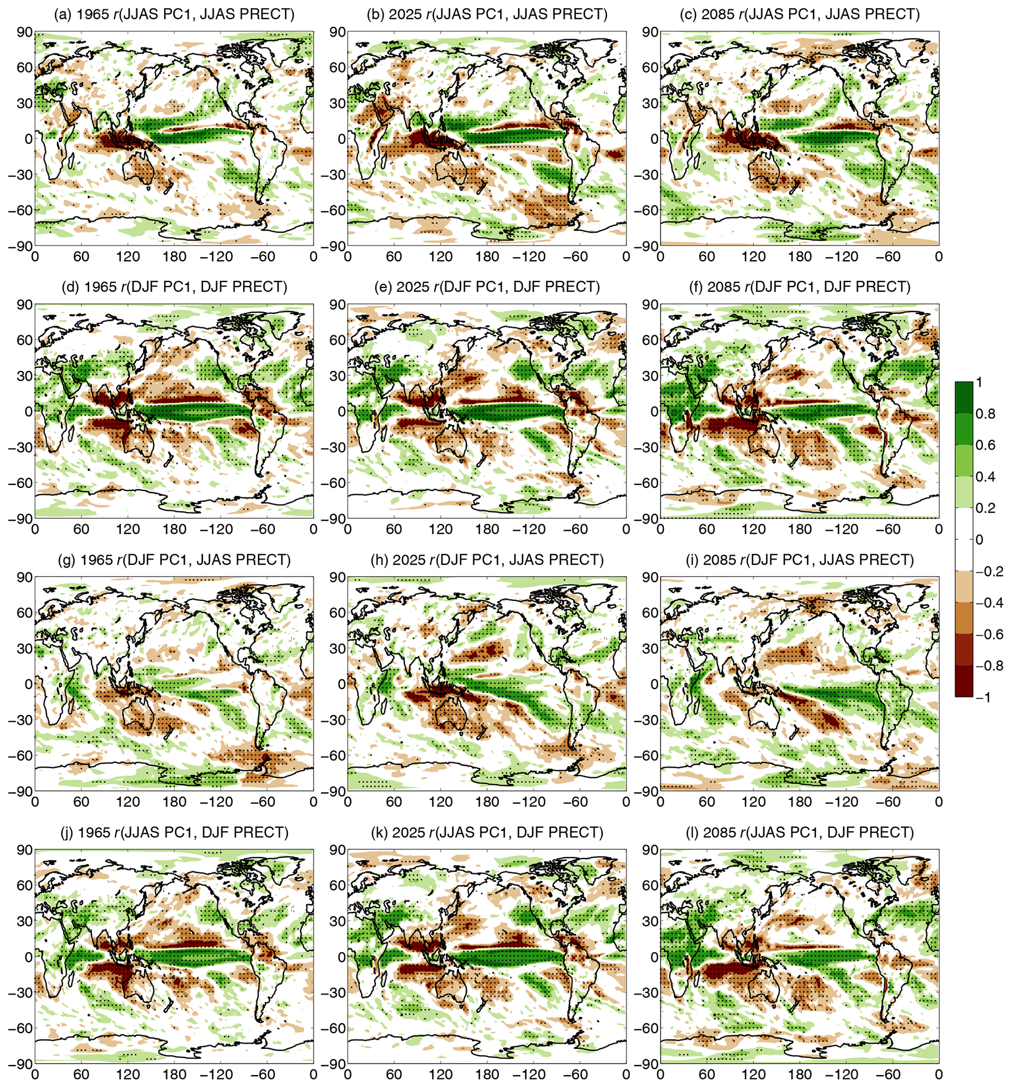
Figure 4Ensemble-based correlation coefficient r maps for the (a–c) JJAS PC1 and JJAS PRECT, (d–f) DJF PC1 and DJF PRECT, (g–i) DJF PC1 and JJAS PRECT, and  (j–l) JJAS PC1 and DJF PRECT. Specific years are indicated in the panels. Dots represent geographical locations where the correlation coefficient is significant at the 95 % level. For better visibility, only every fourth grid point is dotted.

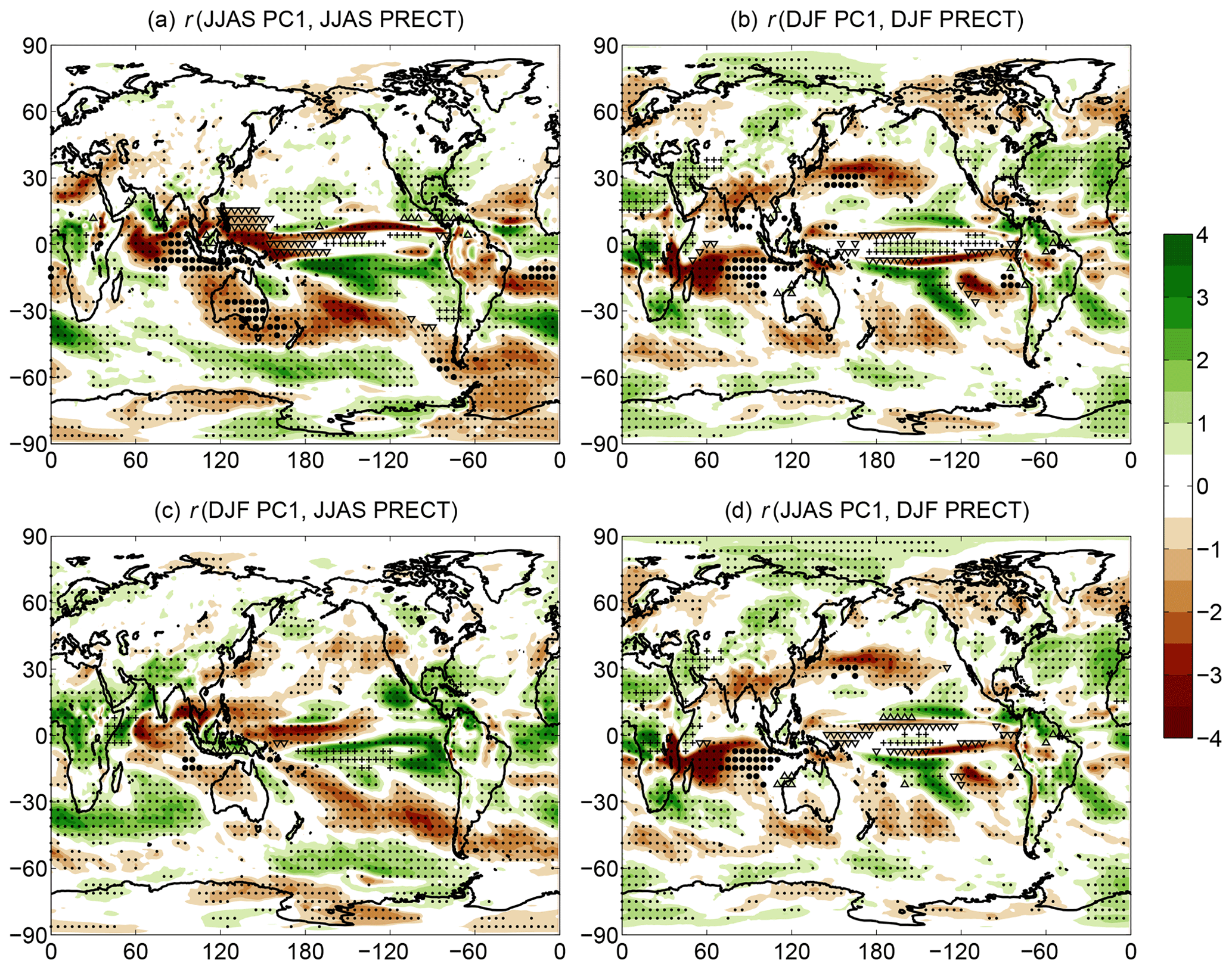
Figure 5The slope of the linear fits (10⁻³ yr⁻¹) at each grid point for the correlation coefficient r for the (a) JJAS PC1 and JJAS PRECT, (b) DJF PC1 and DJF PRECT, (c) DJF PC1 and JJAS PRECT, and (d) JJAS PC1 and DJF PRECT. Dots represent geographical locations where the trend is significant at the 95 % level. In addition, (i) where the trend is positive and the correlation coefficients are positive and significant at the 95 % level in the temporal mean, “+” signs are displayed, (ii) where the trend is positive and the correlation coefficients are negative and significant at the 95 % level in the temporal mean, “△” signs are displayed, (iii) where the trend is negative and the correlation coefficients are positive and significant at the 95 % level in the temporal mean, “▿” signs are displayed, and (iv) where the trend is negative and the correlation coefficients are negative and significant at the 95 % level in the temporal mean, “•” signs are displayed, respectively. For better visibility, the significance and direction of the trend is indicated at only every fourth grid point.

In Fig. 4 these r maps are presented. Four different combinations of PC1 and PRECT correlations are analyzed. The simultaneous (zero lag) correlation between the JJAS data in Fig. 4a–c shows that there are places where the correlation is remarkably negative, indicating dryer conditions during warm events and wetter weather during cold episodes. It is typically observable for Indonesia and Australia, $r\approx (-\mathrm{0.5})$ – (−0.8), eastern Africa, $r\approx (-\mathrm{0.4})$ – (−0.6), Central America, $r\approx (-\mathrm{0.4})$ – (−0.6), the northern part of South America, $r\approx (-\mathrm{0.4})$ – (−0.6), and southern and western parts of India, $r\approx -\mathrm{0.4}$. At the same time positive correlations, indicating more than average precipitation during El Niño and less than average for La Niña, can be seen for northern Africa (r≈0.4) and the west coast of the United States (r≈0.3–0.6). The above-presented picture is roughly consistent with observation-based investigations, see, e.g., Diaz et al. (2001).

It is worth assessing other variations in PC1 and PRECT correlations. The zero-lag correlation between DJF PC1 and DJF PRECT can be seen in Fig. 4d–f. The anticorrelation with $r\approx (-\mathrm{0.4})$ – (−0.8) for southern India, Indonesia, and Australia still holds, as well as the positive correlation for the west coast of the USA, while the eastern African correlation changes sign. In general, the DJF correlation patterns are also fairly close to the observation-based ones, which were reported, e.g., in Diaz et al. (2001), Yang and DelSole (2012), and Yeh et al. (2018).

The role of the lagged correlations is also a relevant issue. It is known that lagged correlation is especially essential, e.g., for the Indian summer monsoon, due to the potential monsoon forecasting (Wu et al., 2012; Johnson et al., 2017; Kucharski and Abid, 2017). Therefore, we construct the ensemble-based lagged correlation maps using the DJF PC1 and JJAS PRECT correlation (Fig. 4g–i). The negative correlation appearing in observations for Indian JJAS precipitation with DJF ENSO phase (Wu et al., 2012) seems to be quite weak in CESM-LE; only a part of southern India has some anticorrelation. This means that in CESM-LE the Indian summer monsoon does not seem to be predictable by the DJF PC1 of the ENSO. In contrast to this, as in the previous cases, the amount of JJAS Indonesian and Australian precipitation shows a clear negative relationship with the DJF PC1. By examining the correlation between the JJAS PC1 and the following DJF PRECT we get interesting results (Fig. 4j–l). India, the mainland of Southeast Asia, and Indonesia show a quite strong anticorrelation, $r\approx (-\mathrm{0.4})$ – (−0.8), while from the northern part of the Indian Ocean through the eastern and central parts of Africa and northward to the Arabian Peninsula a considerable positive correlation can be observed. This suggests that based on the JJAS PC1, as an index for the actual ENSO phase, the DJF precipitation conditions are mostly predictable in these regions.

The question of whether climate change has an impact on the strength of the teleconnections in these regions naturally arises. To answer the question, similarly to the trends obtained for the regression maps in Fig. 2, we construct global linear trend maps of the ensemble-based correlation coefficient maps over time (Fig. 5). For the zero-lag correlations in JJAS (Fig. 5a), among those regions where the strength of the connections are high during the investigated 150 years (indicated by different markers), Australia, an extended part of Indonesia, and the southern part of South America show a clear increase of (1–2)$\times {\mathrm{10}}^{-\mathrm{3}}$ yr⁻¹ in the anticorrelation, while some spots in the southern part of the Atlantic Ocean and central Africa have an increasing positive correlation during 1950–2100; that is, a strengthening of the connection between the phase of the ENSO and the precipitation conditions is found for these regions. Southern India's and Central America's positive correlations and the negative correlation of the Philippine Sea seem to weaken. For the zero-lag correlation in DJF (Fig. 5b) a somewhat different picture opens up. The strength of the positive correlation from central Africa to the Aral Sea and in the North Atlantic Ocean and the strength of the negative correlation in southern India increase further by a trend of (1–4)$\times {\mathrm{10}}^{-\mathrm{3}}$ yr⁻¹, and in the Niño3 region a somewhat stronger positive trend can be found than in JJAS. The spatial distribution of the correlation coefficients is similar for the JJAS PC1 and DJF PRECT (Fig. 2d). The lagged correlations for DJF PC1 and JJAS PRECT (Fig. 5c) are found to increase considerably near the eastern coast of Africa, in the Niño3 and Niño4 regions and around the Caribbean Islands. Thus, based on the larger value of the correlation coefficient implying a stronger relationship, we conclude that a half-year-forward estimate of the precipitation from PC1 data in these regions becomes more accurate. The abovementioned (1–4)$\times {\mathrm{10}}^{-\mathrm{3}}$ yr⁻¹ trends lead to a remarkable change of 0.15–0.45 in the r values over 150 years.