the Creative Commons Attribution 4.0 License.
the Creative Commons Attribution 4.0 License.
 | 11 Feb 2020
A multi-model analysis of teleconnected crop yield variability in a range of cropping systems
Joseph H. A. Guillaume
Christoph Müller
Toshichika Iizumi
Climate oscillations are periodically fluctuating oceanic and atmospheric phenomena, which are related to variations in weather patterns and crop yields worldwide. In terms of crop production, the most widespread impacts have been observed for the El Niño–Southern Oscillation (ENSO), which has been found to impact crop yields on all continents that produce crops, while two other climate oscillations – the Indian Ocean Dipole (IOD) and the North Atlantic Oscillation (NAO) – have been shown to especially impact crop production in Australia and Europe, respectively. In this study, we analyse the impacts of ENSO, IOD, and NAO on the growing conditions of maize, rice, soybean, and wheat at the global scale by utilising crop yield data from an ensemble of global gridded crop models simulated for a range of crop management scenarios. Our results show that, while accounting for their potential co-variation, climate oscillations are correlated with simulated crop yield variability to a wide extent (half of all maize and wheat harvested areas for ENSO) and in several important crop-producing areas, e.g. in North America (ENSO, wheat), Australia (IOD and ENSO, wheat), and northern South America (ENSO, soybean). Further, our analyses show that higher sensitivity to these oscillations can be observed for rainfed and fully fertilised scenarios, while the sensitivity tends to be lower if crops were to be fully irrigated. Since the development of ENSO, IOD, and NAO can potentially be forecasted well in advance, a better understanding about the relationship between crop production and these climate oscillations can improve the resilience of the global food system to climate-related shocks.
- Article
(4611 KB) -
Supplement
(15453 KB) - BibTeX
- EndNote


Climate oscillations are periodically fluctuating oceanic and atmospheric phenomena, and they have been shown to impact hydroclimatological conditions (Dai et al., 1998; Hurrell et al., 2003; Saji and Yamagata, 2003; Trenberth, 1997; Ummenhofer et al., 2009; Ward et al., 2014) and crop productivity (Anderson et al., 2017; Ceglar et al., 2017; Heino et al., 2018; Iizumi et al., 2014; Yuan and Yamagata, 2015) worldwide. The most notorious climate oscillation, the El Niño–Southern Oscillation (ENSO), is the most significant driver of global climate variability (Trenberth, 1997), while two other prominent and widely studied climate oscillations, the Indian Ocean Dipole (IOD) (Saji et al., 1999) and the North Atlantic Oscillation (NAO) (Hurrell, 1995), are also known to affect temperature and precipitation patterns around the globe (Hurrell et al., 2003; Saji and Yamagata, 2003).
All three of these climate oscillations have been shown to significantly impact crop productivity in global (Heino et al., 2018; Iizumi et al., 2014) and regional studies (Anderson et al., 2017; Ceglar et al., 2017; Yuan and Yamagata, 2015). The IOD, for example, strongly affects Australia's drought patterns (Ummenhofer et al., 2009) and crop production (e.g. wheat; Yuan and Yamagata, 2015), while NAO has been shown to particularly impact crop productivity in Europe (Ceglar et al., 2017), but also in the Middle East, northern Africa, and some parts of Asia (Heino et al., 2018; Wang and You, 2004). However, the largest fingerprint of these three oscillations is that of ENSO, which has been found to influence crop productivity on all continents that produce crops (Anderson et al., 2019; Iizumi et al., 2014).
As the phase and development of ENSO, IOD, and NAO can potentially be forecasted from several months (IOD, NAO; Luo et al., 2008; Scaife et al., 2014) up to 1 year (ENSO; Luo et al., 2005; Ludescher et al., 2014) in advance, considerable possibilities arise from understanding the impacts of these climate oscillations on crop production. If these impacts were better understood, it would allow national food agencies, international aid organisations, and food industries and farmers to prepare for varying crop development conditions. This would yield great benefits in increasing the resilience of the global food system to climate-related shocks.
Until now, global-scale studies about the relationship between crop production and climate oscillations have relied on individual satellite-based (Iizumi et al., 2014) or single-model-simulated (Heino et al., 2018) crop yield estimates. The data produced and published in phase 1 of the global gridded crop model intercomparison (GGCMI) of the Agricultural Model Intercomparison and Improvement Project (AgMIP) now allows for the conducting of assessments related to crop yield variability with an ensemble of models and a range of fertiliser use and irrigation set-ups (Elliott et al., 2015; Müller et al., 2019). Given the large variation in crop yield estimates across models (Müller et al., 2017; Rosenzweig et al., 2014), using an ensemble of models can allow for more robust estimates with a better quantification of uncertainty in estimated yield impacts than using a single model.
By using the historical crop yield output derived from a multi-model ensemble of GGCMI, we aim to analyse the impacts of ENSO, NAO, and IOD on maize, rice, soybean, and wheat yields at the global scale. This extends previous studies, which are based on crop yield estimates from single datasets (Heino et al., 2018; Iizumi et al., 2014) and have solely assessed the impacts of ENSO (Iizumi et al., 2014) or the impacts of multiple oscillations on an aggregated crop productivity proxy (Heino et al., 2018). Further, since it is well known that agricultural management can have a major influence on climate-induced crop yield variations (Challinor et al., 2014; Müller et al., 2018), we assess these impacts in different irrigation and fertiliser use scenarios. As a result, we are able to highlight potential management options to mitigate the impacts of these oscillations on crop production. In the “Results and interpretation” section we also compare our results with previous work in order to provide a comprehensive overview of known phenomena while avoiding repetition.
2.1 Physically simulated crop yield data
Global data for physically simulated maize, rice, soybean, and wheat yield (t ha−1) were obtained from the global gridded crop model (GGCM) simulations included in phase 1 of the GGCMI of AgMIP (Elliott et al., 2015; Müller et al., 2019). While most of the 12 models included here simulate the growth of all four target crops, a few simulate only some (Table 1): EPIC-TAMU (maize and wheat), pAPSIM (maize, soybean, and wheat), and PEGASUS (maize, soybean, and wheat). A recent study evaluated the performance of the models included in the GGCMI of AgMIP in reproducing reported historical yield anomalies and did not find any GGCM clearly superior to any other (Müller et al., 2017; Fig. S1 in the Supplement), thus highlighting the benefits of utilising a model ensemble in yield variability assessments to account for uncertainty in individual model results.
Table 1Crop yield data used in this study. “All” refers to all of the crops included in this study, i.e. maize (M), rice (R), soybean (S), and wheat (W). Three model configurations were utilised: harmonised growing season and nutrient input (fullharm), harmonised growing season and no nutrient limitation (harm-suffN), and standard model-specific assumptions (default). Details about the climate forcing data availability are given in the footnotes.
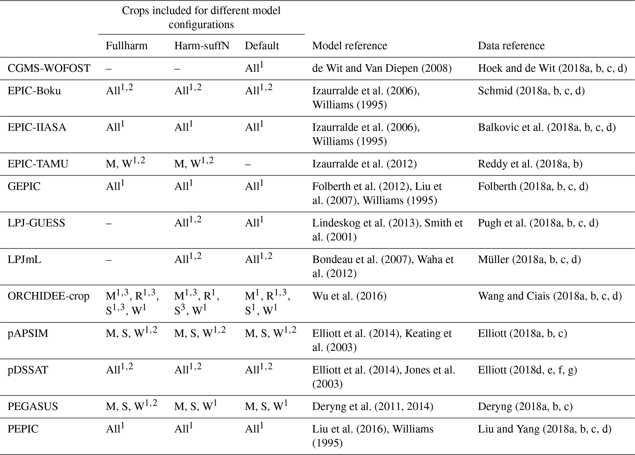
1 AgMERRA, time span: 1980–2010; 2 Princeton, time span: 1948–2008; 3 Princeton, time span: 1979–2010.
Yield variability in the GGCMs included in GGCMI is mainly driven by weather circumstances and CO2 concentration, while soil conditions and agricultural management practices are considered static (Müller et al., 2019). To account for varying assumptions of growing season and fertiliser use, in GGCMI, model simulations were conducted for three configurations: standard model assumptions (default), harmonised growing season and nutrient input (fullharm), and harmonised growing season with no nutrient limitation (harm-suffN). For the default configuration each modelling group used their own model assumptions. In the harmonised model set-ups, crop planting and harvesting dates were standardised among the models and are literature based (Elliott et al., 2015), while fertiliser application rates are either unlimited (harm-suffN) or based on published data (fullharm). Further, all of the GGCMI simulation results are provided separately for irrigated and rainfed conditions. In the irrigated simulation settings, no restrictions on water availability are considered (Müller et al., 2019). In GGCMI, the models simulate only a single growing season per year. Two models included in the GGCMI archive, PRYSBI2 and CLM-Crop, were excluded from this study because either the harmonisation of the growing season provided unreliable results (CLM-Crop) or the model does not distinguish between rainfed and irrigated crops (PRYSBI2).
The “actual” cropping scenario, used in the main analyses (with literature-based shares of rainfed and irrigated areas; see Sect. 2.3), utilises the fullharm set-up and the harm-suffN setting for LPJ-GUESS and LPJmL, which do not consider nitrogen limitation and thus cannot harmonise on fertiliser settings (Table 2). For comparison, the sensitivity analysis (see Sect. 2.4) for the actual cropping scenario was repeated with the default model set-up (see the Supplement), while the harm-suffN scenario was used to assess the impacts of the oscillations in fully fertilised conditions.
Table 2The management scenarios used in this study. The actual set-up is used in the main analyses, while the fully irrigated, rainfed, fully fertilised, and fully irrigated and fertilised management scenarios are used for comparing the impacts in different cropping systems.
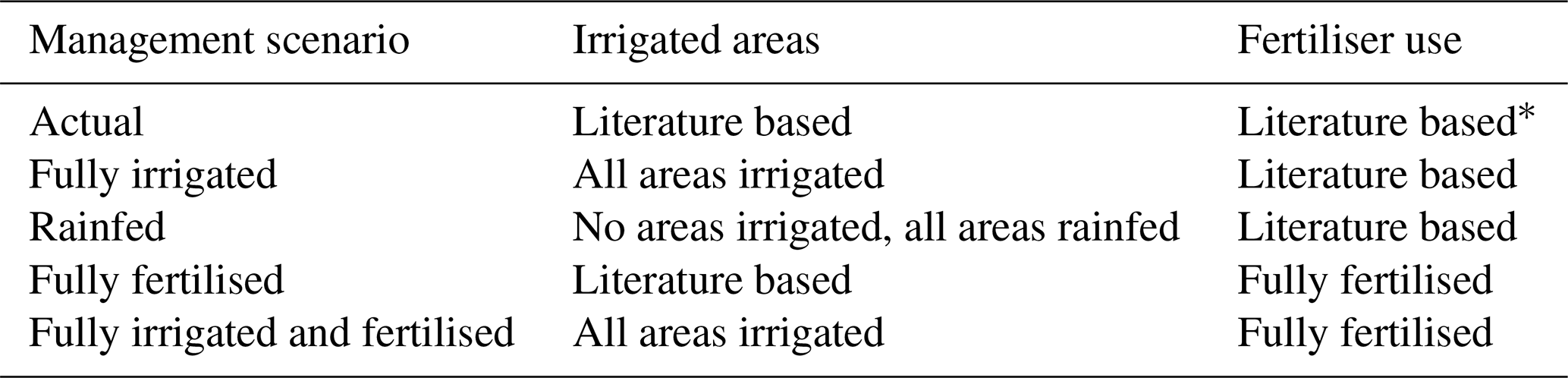
* For LPJ-GUESS and LPJmL, limitations on fertiliser use are not considered. These models are excluded from the “actual” scenario for the comparison with varying fertiliser use.
This study utilises simulations driven with two historical meteorological forcing datasets (bias-corrected reanalysis weather datasets): AgMERRA (Ruane et al., 2015) and the Princeton Global Forcing dataset (Sheffield et al., 2006) (Table 1). AgMERRA was selected as the main climate input for this study, as a large number of GGCMs supplied data for this climate forcing dataset, while the Princeton data were selected for reference due to their long time span and previous use in a similar study (Heino et al., 2018). A detailed description of the GGCMI phase 1 modelling protocol can be found in Elliott et al. (2015), and the output dataset is described by Müller et al. (2019).
2.2 Climate oscillation data
To represent the historical fluctuations of ENSO, IOD, and NAO, the following indices were chosen: the Japan Meteorological Agency (JMA) SST index (Florida State University, 2018), the SST Dipole Mode Index (NOAA Earth System Research Laboratory, 2018; Saji et al., 1999), and Hurrell's North Atlantic Oscillation Index (primary component (PC) based) (Hurrell, 1995; National Center for Atmospheric Research, 2018), respectively. These indices were selected because they are all well established and have already been used in several studies related to crop production (Heino et al., 2018; Kim and McCarl, 2005; Yuan and Yamagata, 2015). For ENSO, the Niño 3.4 index (NOAA Earth System Research Laboratory, 2019) was also tested given its common use in ENSO-related studies (Stuecker et al., 2017; Zhang et al., 2015), with results shown in the Supplement. The indices were transformed to annual values by calculating the mean index for the months when the oscillations tend to have the strongest signal according to existing sources: i.e. December (year t), January (t+1), and February (t+1) for ENSO (Trenberth, 1997) and NAO (Hurrell et al., 2003); September, October, and November (year t for all) for IOD (Saji et al., 1999). This therefore only tests for relationships with a phase-locked measurement of the oscillation rather than investigating intra-annual temporal effects. Using seasonal or monthly data increases the number of significance tests for a given location and therefore the risk of false positives, and interpretation of the results would require an understanding of how climate oscillations, local weather conditions, and yield are connected over time. However, it requires accurate, high-resolution global crop calendars which are not available. Finally, in order to make the oscillation indices comparable with each other, each oscillation index time series was standardised (by subtracting the average index value from the annual values and dividing by their standard deviation).
2.3 Crop yield data aggregation and de-trending
The gridded crop yields were allocated to annual yields based on the sowing dates used in the harmonised GGCMI simulations. The harvest year t is assigned to crop yields which are sown between May of the actual year (t) and April of the next year (t+1). This definition for harvest years was selected because it ensures that the average lifespans of all these oscillations are within the harvest year, and thus many of the major known teleconnections of these oscillations during the crop growing season are included in the analysis (e.g. in Australia, Africa, and South America).
The crop yield data were aggregated spatially to the geographical scale of food production units (FPUs), which divide the world into 573 spatial units that are hybrids of river basins and administrative (economic) areas (Kummu et al., 2010). For the actual cropping scenario, rainfed and irrigated crop yields were combined by calculating the mean yield as the total production divided by the total harvested area across both cropping systems using literature-based values for harvested area (Portmann et al., 2010). The aggregation for fully irrigated and rainfed scenarios was conducted similarly by dividing total production by harvested areas but assuming that all cropland is either irrigated or rainfed, respectively.
In order to extract the interannual variability of the crop yield data, they were de-trended. This was conducted by subtracting a 5-year moving average yield from the annual yield values (3-year average at both ends of the time series), similarly to several previously conducted studies about yield variability (Iizumi et al., 2014; Iizumi and Ramankutty, 2016; Müller et al., 2017, 2018). The anomalies were then divided by 5-year (or 3-year) averages to obtain the proportional annual deviation from the normal values. The equation of the procedure is shown below:
where denotes the relative yield anomaly for each FPU (f), scenario (s), model (m), crop (c), and year (t) compared to the average yield () for the moving time window around year t. The use of a shorter time window at the beginning and end of the yield time series allows for longer de-trended time series, and it is assumed that it would rarely lead to errors in the sign of yield anomalies and thus the derived relationships between climate oscillation and yield anomalies. Other studies have tested other de-trending methods as well but have found no major impact from the method selected (Iizumi et al., 2014; Iizumi and Ramankutty, 2016; Müller et al., 2017).
2.4 Crop yield sensitivity to the oscillations
The sensitivity of actual crop yield to the oscillations was investigated using a multivariate linear regularised ridge regression model, with the oscillation indices as explanatory variables and the annual crop yield anomalies as the dependent variable. The ridge regression framework was selected because it allows correlations among the explanatory variables to be accounted for (here oscillation indices). For the main analysis (actual scenario), the regression was calculated for each FPU separately using crop yield anomaly time series from all GGCMs that simulate the crop in question with the AgMERRA climate input (N=216–297, depending on crop). Hence, we utilise the crop yield time series of all the models in fitting the regression. In the regression model, the slope coefficients represent sensitivity. The optimal regularisation value for the regression was selected by performing a generalised cross-validation (tested regularisation values ranged between 10−6 and 10).
The existence of significant relationships was assessed by calculating a multivariate ridge regression from random bootstrap samples (N=1000, with replacement) of crop yield–oscillation index combinations. Statistical significance therefore tests the robustness of observed ridge regression coefficients across different samples drawn from the time series. The optimal regularisation value was selected for each bootstrap sample as described above, which follows the principle described in Abram et al. (2016). The linear relationship was defined to be significant (p<0.1) if 95 % (two-sided test) of the sampled sensitivity values were either larger or smaller than zero. Thus, a 10 % probability was accepted of wrongly classifying a linear relationship as significant. Note that the relatively high risk level in statistical regression (p<0.1) is commonly used in global climate-yield analysis because of the limited access to high-quality yield data at the global scale (e.g. Ray et al., 2015). To check the robustness of the results, the same analysis was also conducted utilising the crop yield data derived using the Princeton climate input, different model configurations, and individual models and average weather (soil moisture and temperature) conditions (Martens et al., 2017; Ruane et al., 2015) during the growing season. Further, to illustrate the effect of using phase-locked indices rather than investigating intra-annual temporal variation (see Sect. 2.2), the sensitivity of crop yield to these oscillations was also assessed by using the average harvest season oscillation indices as an explanatory variable (see the Supplement).
2.5 Average crop yield anomalies during strong oscillation phases
The crop-specific average yield anomalies observed during strong oscillation phases were investigated for the actual cropping scenario. The crop yield changes that occur during years when the oscillations are in their strong phases were summarised by the median crop yield anomaly (in percent) of those years. The median anomaly was calculated using all the GGCMs that simulate the crop in question (N=216–297, depending on crop) for the actual scenario with AgMERRA climate input. Strongly negative (positive) phases of the oscillations were defined as the years when the respective oscillation index was smaller (larger) than the 25th (75th) percentile of all yearly index values (Nanomaly=54–74, depending on crop). The statistical significance (p<0.1) of the changes was assessed by bootstrapping (n=1000, with replacement) the crop yield anomalies and calculating the median of each bootstrap sample. If over 95 % (two-tailed test) of the sample of medians was either larger or smaller than zero, the change was considered statistically significant. Statistical significance therefore tests the robustness of observed anomalies across different samples drawn from the time series.
2.6 Impacts in different cropping systems
To assess how expanding or reducing the extent of irrigated area and increasing fertiliser use would change the impacts of climate oscillations on crop yields compared to the actual scenario, the main sensitivity analysis (see the description above – Sect. 2.4) was conducted for a set of scenarios (Table 2): (i) all cropland was only rainfed (with fullharm set-up), (ii) all cropland was fully irrigated (fullharm), (iii) all cropland was fully fertilised (actual irrigation with fullharm-suffN), and (iv) all cropland was fully irrigated and fertilised (fully irrigated with harm-suffN). In addition to analysing how the abovementioned four scenarios compare against the actual scenario, the fully irrigated and rainfed scenarios were also compared. To quantify how the impacts in these cropping systems vary, average sensitivity magnitudes were compared for each crop. Specifically, for a pair of scenarios, the average difference of their absolute sensitivity values was calculated across all oscillations and FPUs, whereby at least one of the scenarios shows a significant sensitivity. To obtain a measure relative to the actual (or irrigated when comparing irrigated and rainfed scenarios) scenario, the average difference values were divided with the average sensitivity magnitude of the actual (or irrigated) scenario for the FPUs included. The corresponding equation is
where or is statistically significant; f, s ∈ {s1, s2}, c, and o are indices of FPU, management scenario, crop, and oscillation, respectively. ΔSs12,c denotes the average proportional sensitivity difference of each crop (c) between the scenarios, while and represent the sensitivity in the respective management scenarios s1 and s2; nF,O is the number of cases (oscillation and FPU) in which at least one of the scenarios has a significant sensitivity.
For each crop, to assess whether the mean sensitivity magnitude difference is statistically significantly different from zero, a distribution of the mean sensitivity magnitude difference was created by calculating the average from the bootstrapped (N=1000, with replacement) difference values of each FPU and oscillation. For the comparisons with varying fertiliser use, only the nine GGCMs which have data for both the fullharm and harm-suffN settings, and thus simulate nutrient stress (Table 1), were included.
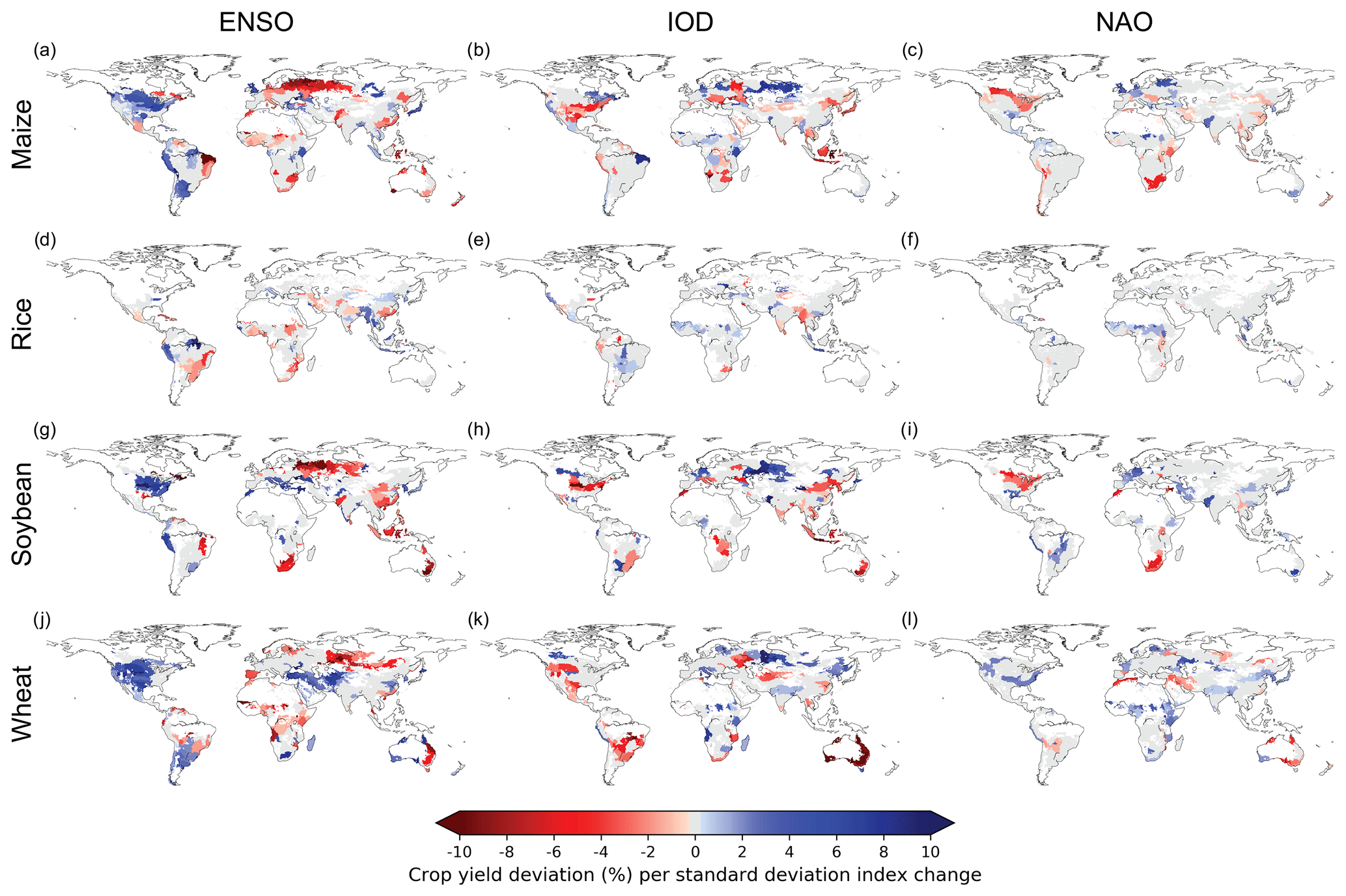
Figure 1Actual maize (a–c), rice (d–f), soybean (g–i), and wheat (j–l) yield sensitivity to ENSO, IOD, and NAO at the FPU scale. The sensitivity values are derived using crop yield data from all GGCMs that simulate the crop in question with the AgMERRA climate input. Statistically insignificant (p>0.1) sensitivity values are marked as zero (grey). White denotes that the crop in question is not produced in that area. Results with Princeton climate input and default model set-up are shown in Figs. S4 and S5, respectively. Median, maximum, and minimum sensitivities as well as consistency across individual models are shown in Figs. S7–S10, respectively. Results for individual models are shown in a zip file in the Supplement. Results with oscillation indices calculated in the harvest season are shown in Fig. S11, with the associated seasons shown in Fig. S12.
3.1 Global extent of climate oscillation impacts
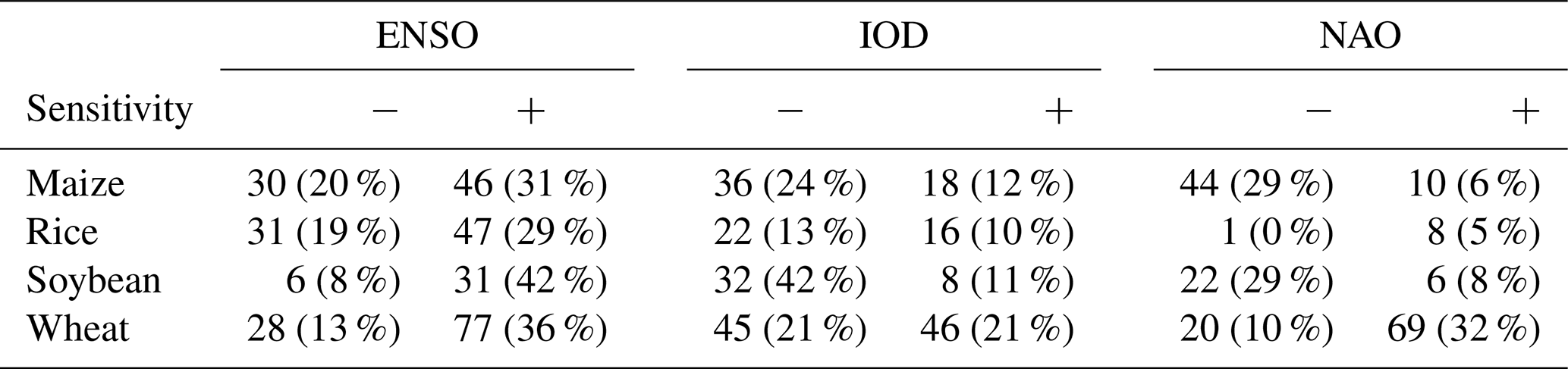
Globally, climate oscillations have widespread effects on crop yields (Table 3), but both the direction and magnitude of impacts vary spatially and across crops (Fig. 1). Out of the oscillations studied here, ENSO shows the widest impacts on yields of maize (statistically significant sensitivity in 51 % of harvested areas), wheat (49 %), and rice (48 %), while IOD and ENSO both show a similar extent of impacts on the yields of soy (53 % and 50 %, respectively) (Table 3). Generally, NAO seems to have the smallest impacts on the yields of the crop types inspected here in terms of harvested areas, although it still shows a relatively strong influence on wheat (42 %) and maize (35 %) yields. In terms of sensitivity direction, it is notably more widespread for yield to increase towards the positive phase of ENSO (i.e. El Niño) for all crop types inspected here (i.e. positive sensitivity). For IOD and NAO, the results are more mixed, though both show larger harvested areas where yield decreases towards the positive phase for maize. These results align with crop yield anomalies during strong oscillation phases, as they also show widespread average impacts (Table S2).
Table 3Extent of significant sensitivity. Crop-specific harvested area (106 ha) extent (and percent of total crop-specific harvested area); actual crop yield shows statistically significant positive (+) or negative (−) sensitivity to ENSO, IOD, and NAO; i.e. there is a statistically significant (two-sided p value < 0.1) linear relationship between crop yield anomalies and the studied oscillations (see Methods). Harvested area extent showing significant anomalies is shown in Table S2.
3.2 Impacts in different areas
ENSO's relationship with crop yield seems to provide the most distinct spatial patterns across the crop types, crop models, and oscillations studied here (Figs. 1–3 and S4–S10 in the Supplement). Crop yields tend to decrease towards the positive phase of ENSO (El Niño) in a large proportion of sub-Saharan Africa, as well as eastern parts of South America and Australia, while yields seem to increase towards the positive phase on the coast of Peru and North America (Fig. 1; global regions mapped in Fig. S1). In general, these results align well with the spatial patterns found in existing studies on the Palmer drought severity index (Dai et al., 1998) as well as soil moisture and temperature anomalies (Figs. S2 and S3). Also, in terms of model and methodological agreement, a consistent increase (decrease) in wheat yields in parts of the Middle East can be observed for ENSO towards its positive (negative) phase (Figs. 1–3 and S11–S12). For the southern tip of Africa, wheat and soybean seem to be related with opposite impacts. This is potentially because of differences in harvest timing and the related weather conditions; wheat is harvested in the autumn, while soybean is harvested the following spring and is thus more exposed to the drier conditions related to ENSO during the boreal winter (Fig. S2, Philippon et al., 2012).
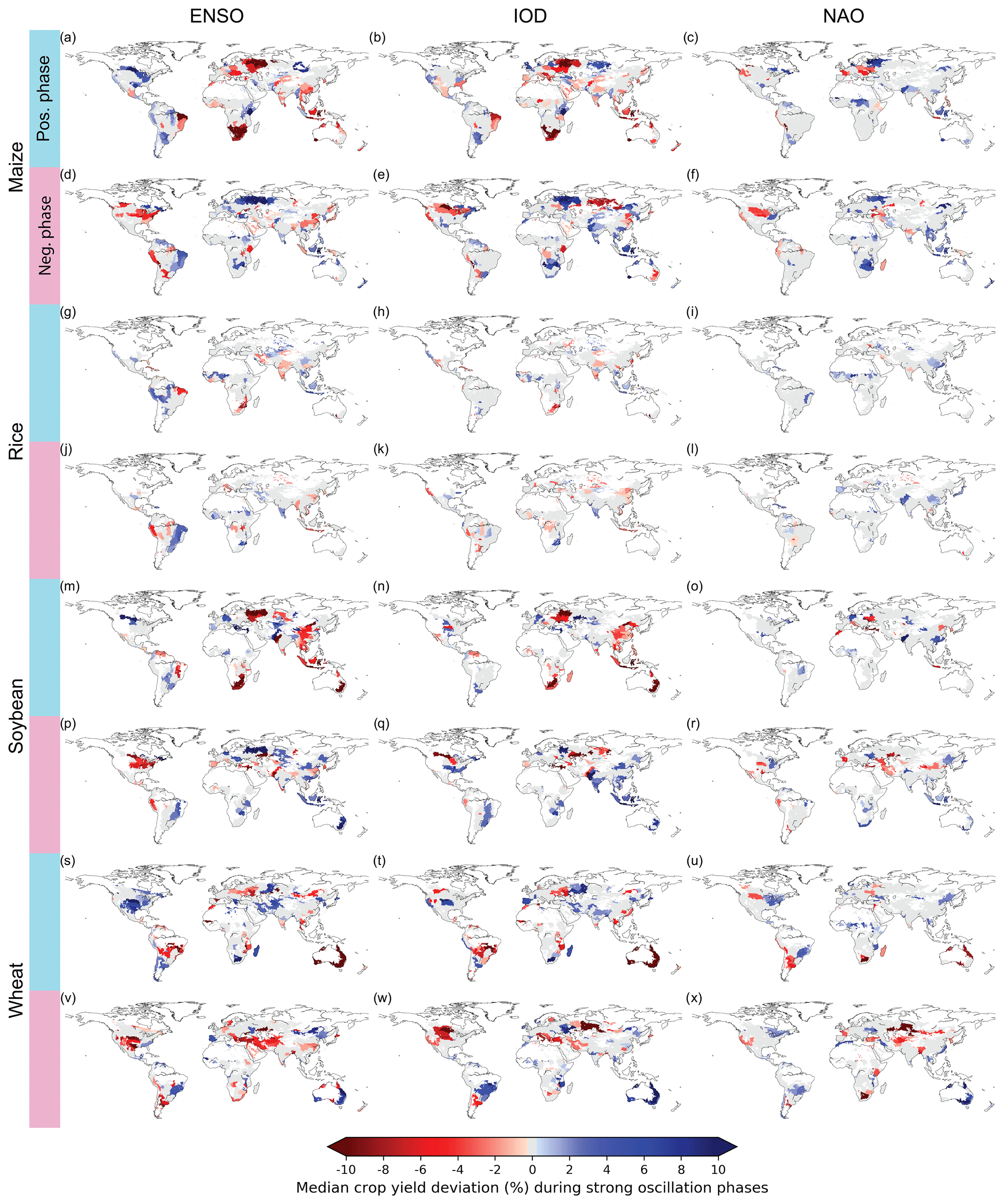
Figure 2Actual maize (a–f), rice (g–l), soybean (m–r), and wheat (s–x) yield anomalies during strong phases of ENSO, IOD, and NAO at the FPU scale. The anomaly values are derived from a sample including crop yield data from all GGCMs that simulate the crop in question with the AgMERRA climate input. Statistically insignificant (p>0.1) anomaly values are marked as zero (grey). White denotes that the crop in question is not produced in that area. Patterns are discussed in Sect. 3.1 and 3.2.
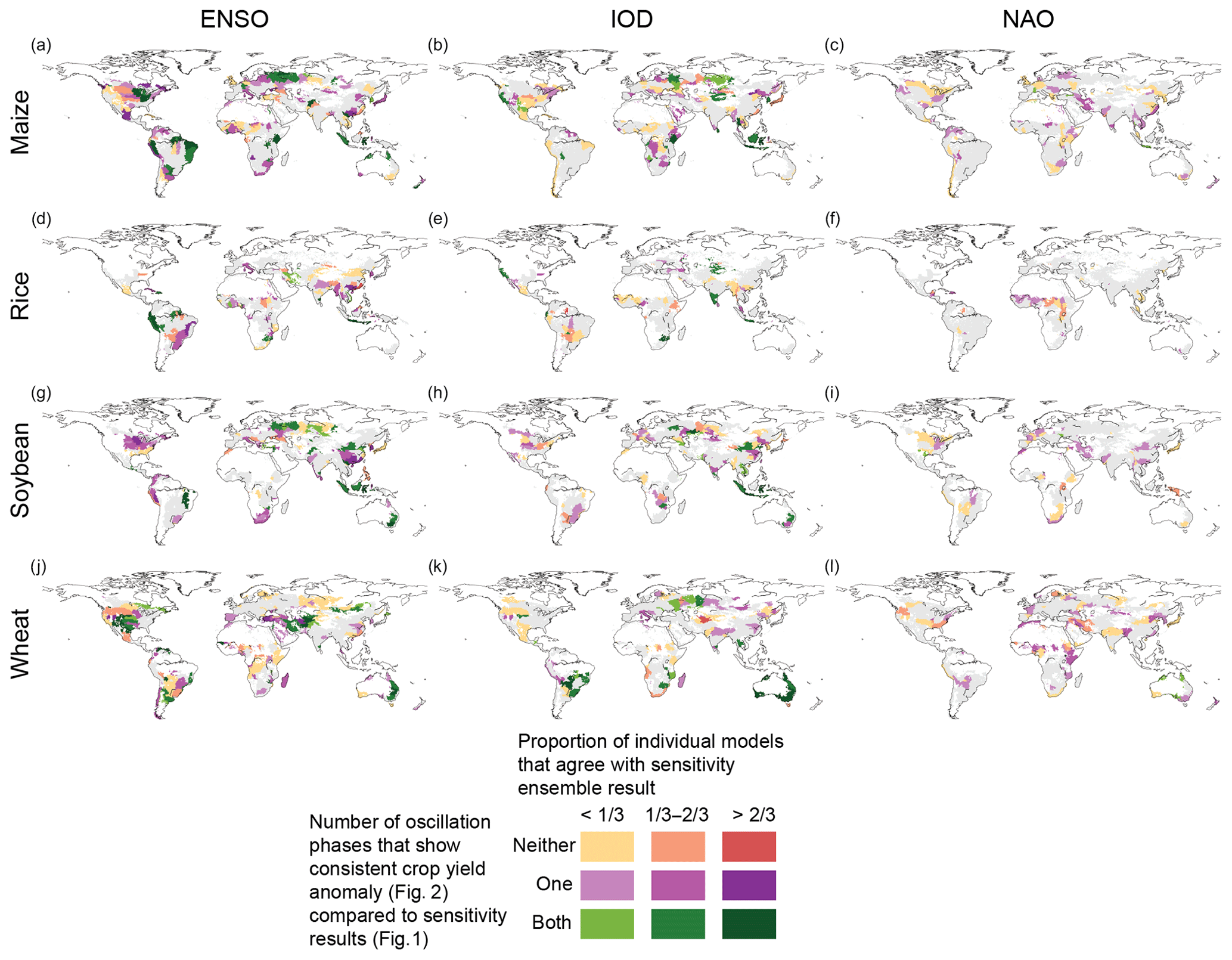
Figure 3Summary of the relationship between ENSO, IOD, and NAO and crop yields across models and methods for maize (a–c), rice (d–f), soybean (g–i), and wheat (j–l). The y axis of the colour bar shows whether there is agreement between the sensitivity analysis (Fig. 1) and the average anomalies during strong oscillation phases (Fig. 2): “neither” denotes that the strong oscillation phases are not related to significant average crop yield anomalies that are consistent with the sensitivity analysis; “one” means that either the positive or negative oscillation phase shows a significant average anomaly that is consistent with the sensitivity result (e.g. positive sensitivity and positive anomaly during a positive oscillation phase); and “both” means that both phases of the oscillations show consistent average anomalies during the strong oscillation phases (e.g. positive anomaly during a positive oscillation phase and negative anomaly during a negative oscillation phase in an FPU with positive sensitivity). The x axis of the colour bar shows the proportion of individual models that show significant sensitivity of the same sign compared to the result from the ensemble analysis (see Fig. 1 above, Fig. S10, and zip files in the Supplement). Areas where the ensemble results do not show a statistically significant relationship are marked in grey, while white denotes that the crop in question is not grown in that area.
When comparing our results to a study about ENSO's crop yield impacts, which utilised satellite-based crop yields (Iizumi et al., 2014, 2018a), the agreement of the impacts varies. Our results agree with existing studies, for example, for large parts of Africa and eastern Asia, where El Niño is mostly related to negative impacts, while results do not agree in North America (wheat, maize) and Australia (maize). However, it should be noted that these differences are no surprise, since it has been shown that only a third of global crop yield variability can be attributed to seasonal climate variation (Ray et al., 2015). In contrast to satellite-based data, the models used here deliberately focus on weather impacts on crop yield and do not consider the impacts of e.g. multiple cropping or weather-triggered pest outbreaks and management responses, which can also be major contributors to crop yield variations.
For IOD, strong and consistent impacts (Figs. 1 and 2) among crop models (Fig. 3) can be observed in eastern Australia, especially for soybean and wheat (Figs. 1–3), where the IOD is related to drier and warmer weather conditions (Figs. S2 and S3). This corroborates a previous study conducted on the relationship between IOD and wheat yields, which showed that around 40 % of Australia's wheat yield variability can be attributed to the IOD (Yuan and Yamagata, 2015); where the oscillations are together it is also able to explain a substantial portion of crop yield variability (>25 %, Fig. S13). Further, consistent results among models and methods (Figs. 1–3) for IOD can be observed in parts of eastern Europe and central Asia, where the positive (negative) phase of the IOD is related to an increase (decrease) in wheat, maize, and soybean yields. In Southeast Asia and southern Africa, the impacts of the IOD vary between crops. For example, in Southeast Asia, rice shows a positive sensitivity (increasing yield towards the positive phase), while maize and soybean show a negative one. In eastern China, maize, wheat, and soybean yield variability seems to be related to the IOD to some extent. However, these relationships are less certain, as they are not consistently found by the majority of the individual models (Fig. 3).
For NAO, the relationships are generally less certain in terms of model agreement compared to ENSO and IOD (Fig. 3). NAO's most significant impacts can be observed in eastern Europe and the Middle East for maize, soybean, and wheat yields (Figs. 1 and 2). In the Middle East, the sensitivity of wheat and maize (soybean) yield to NAO seems to be negative (positive), while mostly positive sensitivity is found in Europe and western Russia for maize, soybean, and wheat. These differences between crop types observed in the Middle East can potentially be due to differing growing seasons. In the models, the sowing dates of soybean vary strongly in space and between irrigation regimes (for some areas soybean sowing occurs in spring before May, while in other areas soybean is planted later in the year), which can have an effect on the observed signal compared to maize and wheat. In general, the patterns observed in eastern Europe, western Russia, and the Middle East align well with results from previous studies about crop productivity and weather variations (Cullen et al., 2002; Heino et al., 2018; Hurrell et al., 2003). Although the results for NAO are relatively similar between different model configurations (Figs. S4 and S5), the results are not as consistent among the GGCMs as for the other oscillations (Fig. 3).
3.3 Magnitude of impacts in different cropping systems
Irrigation plays a key role in reducing crop yield sensitivity to climate oscillations, with yield varying up to 3 times more (for wheat) across the range of oscillations when comparing fully irrigated and rainfed scenarios (Fig. 4). Comparing rainfed to actual conditions shows that irrigation has already substantially reduced the effects of climate oscillations on crop yields. The average difference in sensitivity is the largest for rice, for which the average sensitivity would be over 2 times higher, i.e. the yield would vary 2 times more across the range of the oscillations, if all cropland was rainfed (Fig. 4g). The difference in sensitivity is the smallest for soybean (29 %, Fig. 4l), while maize and wheat show a relative increase in sensitivity of 47 % (Fig. 4b) and 60 % (Fig. 4q), respectively. This ranking is expected, as the majority of rice harvested areas are irrigated (62 % globally) and soybean has the smallest irrigated area share of these four crops (8 %), while maize (21 %) and wheat (31 %) fall in between (Portmann et al., 2010).
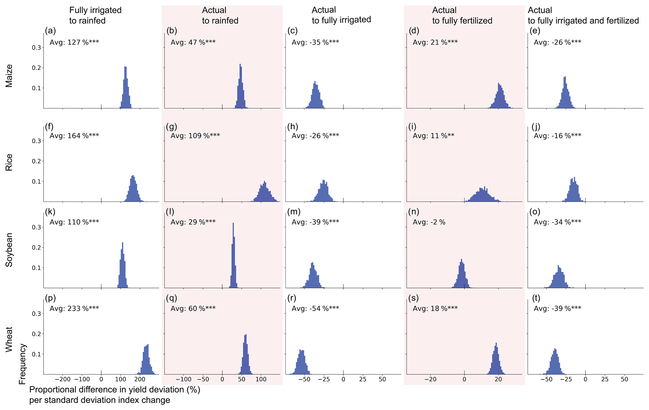
Figure 4Relative average difference in sensitivity magnitude of maize (a–e), rice (f–j), soybean (k–o), and wheat (p–t) between a range of cropping scenarios through all the studied oscillations and FPUs. To quantify how the impacts in these cropping systems vary, average sensitivity magnitudes were compared for each crop. Specifically, for a pair of scenarios, the average difference of their absolute sensitivity values was calculated across all oscillations and FPUs, with at least one scenario showing a significant sensitivity. To obtain a measure relative to the actual (or irrigated when comparing irrigated and rainfed scenarios) scenario, the average difference values were divided with the average sensitivity magnitude of the actual (irrigated) scenario for the FPUs included. For each crop, to assess whether the mean sensitivity magnitude difference is statistically significantly different from zero, a distribution of the mean difference was created by calculating the average from the bootstrapped (N=1000, with replacement) difference values of each FPU and oscillation. For the scenarios with varying fertiliser use set-up, we included only the nine GGCMs which have data for both the fullharm and harm-suffN settings and also simulate nutrient stress, i.e. pDSSAT, EPIC-Boku, EPIC-IIASA, GEPIC, pAPSIM, PEGASUS, EPIC-TAMU, ORCHIDEE-crop, and PEPIC. Triple, double, and single asterisks denote the confidence level at 99.9 %, 99 %, and 90 %, respectively. Maps of sensitivity for each cropping system are shown in Figs. S14–S18 and differences in sensitivity magnitude in Figs. S19–S23. Please note the different scale in the x axis between the columns.
Conversely, average sensitivity would be reduced if crops were fully irrigated without any limitations on water availability compared to the actual situation for all the inspected crop types. The benefits of further irrigation are limited by its current use, which might be why rice shows the smallest difference in average impacts (most of the rice harvested area is already irrigated; Fig. 4h). The average decrease in crop yield sensitivity to the oscillations is the largest for wheat (54 %; i.e. yield varies 54 % less across the oscillations compared to actual conditions – Fig. 4r) and soybean (39 %, Fig. 4m), while maize shows a 35 % (Fig. 4c) average decrease.
Unlimited fertiliser (fully fertilised scenario) use yields statistically significantly larger average sensitivity compared to actual conditions for maize (21 %, Fig. 4d), rice (11 %, Fig. 4i), and wheat (18 %, Fig. 4s). For these crops, these climate oscillations have a stronger impact on yields in cropping systems that do not have limitations related to nutrient availability. This reflects previous research that has found increased crop yield variability under additional fertiliser inputs (Müller et al., 2018). This is potentially because in low-crop-yield years, fertiliser use is not the main limiting factor, so yields are not significantly improved, while in years when climate conditions are suitable for crop growth, yields become even higher, which would increase the sensitivity value as well (Fig. S24). Note that this does not mean fertiliser fails to improve crop yields, only that it does not lead to more stable yields in the face of weather variability. Soybean has very little change in sensitivity under full fertilisation (Fig. 4n). This is likely because it is a legume and has lower nitrogen requirements (nitrogen availability is not even considered in soybean simulations in some models).
Combining both unlimited irrigation and fertilisers, all of the crop types show smaller average sensitivity compared to the actual cropping system scenario (Fig. 4). The decreased sensitivity due to increased irrigation dominates the increased sensitivity due to increased fertiliser use. However, the differences in sensitivity magnitude are large between crops, with wheat having the largest decreases in average sensitivity magnitude (39 %, Fig. 4t) and rice having the smallest (16 %, Fig. 4j).
The abovementioned results can be observed spatially in the Supplement (Figs. S14–S23), which e.g. clearly show that, in most areas, the sensitivity magnitude is larger in the rainfed and fully fertilised scenarios; i.e. yields vary more across the range of the oscillation index. The spatial results also highlight areas with the potential to reduce the impact of oscillations, for example for ENSO in northern South America (soybean and rice) and for IOD in Australia (wheat), where high sensitivity to the respective oscillations can be observed for the actual scenario.
In this study, we inspected the historical relationship between crop yield variability and climate oscillations in a range of cropping systems by utilising an ensemble of historical crop yield simulations generated in GGCMI. The results of this study highlight the widespread impacts that ENSO, IOD, and NAO have on crop yields at the global scale, as well as potential options for mitigating their impacts. Further, we find robust impacts for these oscillations in many areas around the globe, e.g. in North and South America for ENSO and in eastern Australia for IOD, where these insights can potentially be utilised in efforts to mitigate weather-driven variations in crop productivity (Iizumi et al., 2018b).
The reliability and usefulness of these results vary significantly between regions, crops, and oscillations. In general, the teleconnections related to ENSO are the strongest, which is sensible, since ENSO has been shown to be the most significant driver of global climate variability (Dai et al., 1998; Trenberth, 1997). Various institutions (including the United Nations) already provide action plans to mitigate ENSO's impacts on society. In Australia, there is significant potential to utilise the information for IOD along with ENSO to understand crop yield fluctuations, as they can explain a large proportion of local crop yield variability (Fig. S13; Yuan and Yamagata, 2015). Some promise also exists in using oscillation forecasts to predict crop yield variability (Nobre et al., 2019). However, the quality of predictions of this type would naturally depend on the skill of the climate forecasts and the strength of the teleconnection. This study only provides a first assessment of correlations, and further work is needed before reliable forecasts can be provided.
Our results join existing research (Müller et al., 2018; Schauberger et al., 2016; Okada et al., 2018) in highlighting the major role of irrigation in mitigating climate-related crop yield variations and thus securing global food production. This is an important point, since water supplies are highly stressed in many important crop-producing areas (Kummu et al., 2016) which are also impacted by climate oscillations, such as parts of North America and South Asia. Thus, diminishing water resources could pose a major barrier to mitigating future negative impacts related to climate oscillations and climate variability in general. This can be very problematic, given that climate change will likely increase the occurrence of extreme weather in the future (Coumou and Robinson, 2013). With given water shortages in some regions (Heinke et al., 2019), exploiting potentials to improve sustainable water use in agriculture (Jägermeyr et al., 2017) may thus be highly important for maintaining the long-term stability of the global crop production system. It should also be noted that there is substantial potential to improve water use efficiency with integrated crop water management measures (Jägermeyr et al., 2016).
Interestingly, at the global level, increasing fertiliser use does not seem to decrease the sensitivity of crop yields to oscillations, potentially because low-crop-yield years remain the same, while in years when conditions are suitable for crop growth, yields become even higher (Müller et al., 2018), which would increase the sensitivity value as well. This explanation aligns with previous research, which has shown that increasing fertiliser use has limited potential to increase crop yields during years when weather conditions limit crop growth (Liebig's law). In other words, additional fertiliser use in years with unfavourable seasonal climate condition does not lead to yield gain and is not cost effective, even if it is beneficial in normal conditions. Therefore, decision support systems which guide farmers about optimal fertiliser use under the predicted growing season climate can be useful to avoid investments in fertilisers in bad years (Hayashi et al., 2018).
Limitations and way forward
The selection of the time windows for calculating the oscillation metric and defining the related growing seasons can have an impact on the spatial crop yield sensitivity footprint, as briefly illustrated in this study as well (Figs. 1 and S11). Previously used approaches for identifying these relationships include e.g. looking at crop yield anomalies for the year (Heino et al., 2018; Iizumi et al., 2014; Yuan and Yamagata, 2015) and years around (Anderson et al., 2017) strong oscillation anomalies. In these studies, strong oscillation anomalies are calculated either for the season in which the oscillations show their strongest signal (Heino et al., 2018; Anderson et al., 2017; Yuan and Yamagata, 2015) or the harvest season (Iizumi et al., 2014). In general, it can be said that it is very difficult to find metrics for the oscillations that would work perfectly everywhere. A lack of accurate, spatially detailed crop calendars makes addressing this issue particularly challenging. The justification for the methods used here is to look at how crop yields vary around the time at which these oscillations show their strongest signal, which can provide valuable information for early warning systems.
Future work could try to trace intermediate effects in order to explain the mechanisms at play, e.g. combining the effect of oscillations on weather, the effect of each aspect of weather on crop planting, development, and harvest, and the final result in terms of crop yield. Such research could additionally provide useful information for decreasing crop yield variations and thus increasing the resilience of crop production to climate variability.
The teleconnection patterns related to the IOD can be difficult to fully disentangle from ENSO due to their coevolution. Previous studies have shown that around 20 % to 45 % of IOD variability could be explained by ENSO depending on the data and the investigated time frame (Saji and Yamagata, 2003; Zhang et al. 2015). The nature of this relationship is still debated (Hameed et al., 2018; Stuecker et al., 2017), and determining the influence of ENSO on the IOD and vice versa is not in the scope of this study. However, through the use of multivariate ridge regression, we aim to filter the influence of ENSO from the IOD patterns. Also, the relationship between ENSO and NAO has been studied, but that relationship has been shown to be relatively weak (Hurrell et al., 2003).
The data used here are from state-of-the-art global gridded crop models included in phase 1 of the GGCMI of AgMIP. However, major uncertainties in the simulated crop yields still exist, and the relationships observed here between crop yields and these oscillations are often not consistent throughout the ensemble of crop models (see Fig. 3). Differences and uncertainties among the models arise e.g. from soil and crop type parameterisations as well as handling of water and nutrient stress (e.g. Folberth et al., 2019). Additionally, uncertainties in these GGCMs arise from the simulated cropping systems, as simulations assume only a single annual harvest per crop and per grid cell, whereas multiple harvests are common for e.g. rice. In general, simulated crop yields seem to be most reliable in high-nutrient-input areas (Müller et al., 2017), where observed climate variability also explains a majority of reported crop yield variation (Ray et al., 2015).
This study has included comparisons with fully fertilised and irrigated management scenarios intended to capture (unattainable) ideal management, with no water or nutrient stress anywhere. This helps us understand the physical potential of management measures for mitigating the crop yield variability related to these oscillations according to the models used. In future, practical limitations could also be taken into account by limiting water and fertiliser use to locally available resources.
The three climate oscillations included here are only a share of the whole range of periodically fluctuating climatological phenomena that could impact crop growing conditions. Thus, studying the relationship between simulated crop yields and other climate oscillations not included here, such as the Scandinavian pattern or the Arctic Oscillation, would provide additional insights into this topic, as demonstrated in a recent study by Ceglar et al. (2017).
This study strengthens the evidence that climate oscillations are drivers of crop yield variability around the world. In several areas where these oscillations show robust impacts on crop production, e.g. Australia, southern Africa, and parts of North and South America, local risk reduction efforts and global efforts can already benefit from utilising these known relationships to improve stakeholder preparedness against crop production shocks associated with the climate oscillations. Information for maintaining the stability of global crop production is of high importance, given that anticipated climate change and population growth will keep increasing the pressure on the global food system. Finally, our results suggest that increases (decreases) in the extent of irrigated area would, on average, reduce (amplify) the impacts of these oscillations on crop yields, which highlights the importance of sustainable water use in maintaining the long-term stability of the global crop production system.
The processing scripts are available from GitHub: https://github.com/matheino/crops_and_oscillations (last access: 19 September 2019) (Heino, 2019). The simulated crop yield data were retrieved from the GGCMI data archive at: http://www.rdcep.org/research-projects/ggcmi (last access: 11 November 2017) (Center for Robust Decision-making on Climate and Energy Policy, 2017); they are also available through the links provided in the references of Table 1.
The supplement related to this article is available online at: https://doi.org/10.5194/esd-11-113-2020-supplement.
MH, JHAG, and MK designed the research in consultation with CM and TI. Analyses were conducted by MH and supported by all co-authors. MH wrote the article, with contributions from all co-authors.
The authors declare that they have no conflict of interest.
We acknowledge the Agricultural Intercomparison and Improvement Project (AgMIP) for data provision.
This research has been supported by the Academy of Finland (grant nos. 305471 and 317320), the Strategic Research Council (grant no. 303623), the Emil Aaltonen Foundation (project eat-less-water), Maa-ja vesitekniikan tuki ry (Vesi ja kehitys -tohtorikoulu), the AaltoENG doctoral programme, and the Vilho, Yrjö and Kalle Väisälä Foundation as well as the European Research Council (ERC) under the European Union's Horizon 2020 research and innovation programme (grant agreement no. 819202).
This paper was edited by Daniel Kirk-Davidoff and reviewed by Daniel Kirk-Davidoff and one anonymous referee.
Abram, S. V., Helwig, N. E., Moodie, C. A., DeYoung, C. G., MacDonald III, A. W., and Waller, N. G.: Bootstrap Enhanced Penalized Regression for Variable Selection with Neuroimaging Data, Frontiers in neuroscience, 10, 344, 2016.
Anderson, W., Seager, R., Baethgen, W., and Cane, M.: Crop production variability in North and South America forced by life-cycles of the El Niño Southern Oscillation, Agr. Forest Meteorol., 239, 151–165, 2017.
Anderson, W. B., Seager, R., Baethgen, W., Cane, M., and You, L.: Synchronous crop failures and climate-forced production variability, Sci. Adv., 5, eaaw1976, https://doi.org/10.1126/sciadv.aaw1976, 2019.
Balkovic, J., Khabarov, N., and Skalsky, R.: AgMIP's Global Gridded Crop Model Intercomparison (GGCMI) phase 1 output data set: EPIC-IIASA maize, Zenodo, https://doi.org/10.5281/zenodo.1403203, 2018a.
Balkovic, J., Khabarov, N., and Skalsky, R.: AgMIP's Global Gridded Crop Model Intercomparison (GGCMI) phase 1 output data set: EPIC-IIASA rice, Zenodo, https://doi.org/10.5281/zenodo.1403199, 2018b.
Balkovic, J., Khabarov, N., and Skalsky, R.: AgMIP's Global Gridded Crop Model Intercomparison (GGCMI) phase 1 output data set: EPIC-IIASA soy, Zenodo, https://doi.org/10.5281/zenodo.1403197, 2018c.
Balkovic, J., Khabarov, N., and Skalsky, R.: AgMIP's Global Gridded Crop Model Intercomparison (GGCMI) phase 1 output data set: EPIC-IIASA wheat, Zenodo, https://doi.org/10.5281/zenodo.1403195, 2018d.
Bondeau, A., Smith, P. C., Zaehle, S., Schaphoff, S., Lucht, W., Cramer, W., Gerten, D., Lotze-campen, H., Müller, C., Reichstein, M., and Smith, B.: Modelling the role of agriculture for the 20th century global terrestrial carbon balance, Global Change Biol., 13, 679–706, https://doi.org/10.1111/j.1365-2486.2006.01305.x, 2007.
Ceglar, A., Turco, M., Toreti, A., and Doblas-Reyes, F. J.: Linking crop yield anomalies to large-scale atmospheric circulation in Europe, Agr. Forest Meteorol., 240, 35–45, 2017.
Center for Robust Decision-making on Climate and Energy Policy: Global Gridded Crop Model Intercomparison (GGCMI) Project, available at: http://www.rdcep.org/research-projects/ggcmi, last access: 11 November 2017.
Challinor, A. J., Watson, J., Lobell, D. B., Howden, S. M., Smith, D. R., and Chhetri, N.: A meta-analysis of crop yield under climate change and adaptation, Nat. Clim.Change, 4, 287–291, 2014.
Coumou, D. and Robinson, A.: Historic and future increase in the global land area affected by monthly heat extremes, Environ. Res. Lett., 8, 034018, https://doi.org/10.1088/1748-9326/8/3/034018, 2013.
Cullen, H. M., Kaplan, A., and Arkin, P. A.: Impact of the North Atlantic Oscillation on Middle Eastern climate and streamflow, Climatic Change, 55, 315–338, 2002.
Dai, A., Trenberth, K. E., and Karl, T. R.: Global variations in droughts and wet spells: 1900–1995, Geophys. Res. Lett., 25, 3367–3370, 1998.
Deryng, D. AgMIP's Global Gridded Crop Model Intercomparison (GGCMI) phase 1 output data set: PEGASUS maize, Zenodo, https://doi.org/10.5281/zenodo.1409550, 2018a.
Deryng, D. AgMIP's Global Gridded Crop Model Intercomparison (GGCMI) phase 1 output data set: PEGASUS soy, Zenodo, https://doi.org/10.5281/zenodo.1409548, 2018b.
Deryng, D. AgMIP's Global Gridded Crop Model Intercomparison (GGCMI) phase 1 output data set: PEGASUS wheat, Zenodo, https://doi.org/10.5281/zenodo.1409546, 2018c.
Deryng, D., Sacks, W. J., Barford, C. C., and Ramankutty, N.: Simulating the effects of climate and agricultural management practices on global crop yield, Global Biogeochem. Cy., 25, GB2006, https://doi.org/10.1029/2009GB003765, 2011.
Deryng, D., Conway, D., Ramankutty, N., Price, J., and Warren, R.: Global crop yield response to extreme heat stress under multiple climate change futures, Environ. Res. Lett., 9, 034011, https://doi.org/10.1088/1748-9326/9/3/034011, 2014.
de Wit, A. J. and Van Diepen, C. A.: Crop growth modelling and crop yield forecasting using satellite-derived meteorological inputs, Int. J. Appl. Earth Obs. Geoinf., 10, 414–425, 2008.
Elliott, J.: AgMIP's Global Gridded Crop Model Intercomparison (GGCMI) phase 1 output data set: pAPSIM maize, Zenodo, https://doi.org/10.5281/zenodo.1403189, 2018a.
Elliott, J.: AgMIP's Global Gridded Crop Model Intercomparison (GGCMI) phase 1 output data set: pAPSIM soy, Zenodo, https://doi.org/10.5281/zenodo.1403185, 2018b.
Elliott, J.: AgMIP's Global Gridded Crop Model Intercomparison (GGCMI) phase 1 output data set: pAPSIM wheat, Zenodo, https://doi.org/10.5281/zenodo.1403183, 2018c.
Elliott, J.: AgMIP's Global Gridded Crop Model Intercomparison (GGCMI) phase 1 output data set: pDSSAT maize, Zenodo, https://doi.org/10.5281/zenodo.1403181, 2018d.
Elliott, J.: AgMIP's Global Gridded Crop Model Intercomparison (GGCMI) phase 1 output data set: pDSSAT rice, Zenodo, https://doi.org/10.5281/zenodo.1403177, 2018e.
Elliott, J.: AgMIP's Global Gridded Crop Model Intercomparison (GGCMI) phase 1 output data set: pDSSAT soy, Zenodo, https://doi.org/10.5281/zenodo.1403173, 2018f.
Elliott, J.: AgMIP's Global Gridded Crop Model Intercomparison (GGCMI) phase 1 output data set: pDSSAT wheat, Zenodo, https://doi.org/10.5281/zenodo.1403171, 2018g.
Elliott, J., Kelly, D., Chryssanthacopoulos, J., Glotter, M., Jhunjhnuwala, K., Best, N., Wilde, M., and Foster, I.: The parallel system for integrating impact models and sectors (pSIMS), Environ. Model. Softw., 62, 509–516, https://doi.org/10.1016/j.envsoft.2014.04.008, 2014.
Elliott, J., Müller, C., Deryng, D., Chryssanthacopoulos, J., Boote, K. J., Büchner, M., Foster, I., Glotter, M., Heinke, J., Iizumi, T., Izaurralde, R. C., Mueller, N. D., Ray, D. K., Rosenzweig, C., Ruane, A. C., and Sheffield, J.: The Global Gridded Crop Model Intercomparison: Data and modeling protocols for Phase 1 (v1.0), Geosci. Model Dev., 8, 261–277, https://doi.org/10.5194/gmd-8-261-2015, 2015.
Florida State University: ENSO Index According to JMA SSTA, available at: https://www.coaps.fsu.edu/jma, last access: August 2018.
Folberth, C.: AgMIP's Global Gridded Crop Model Intercomparison (GGCMI) phase 1 output data set: GEPIC maize, Zenodo, https://doi.org/10.5281/zenodo.1408577, 2018a.
Folberth, C.: AgMIP's Global Gridded Crop Model Intercomparison (GGCMI) phase 1 output data set: GEPIC rice, Zenodo, https://doi.org/10.5281/zenodo.1408575, 2018b.
Folberth, C.: AgMIP's Global Gridded Crop Model Intercomparison (GGCMI) phase 1 output data set: GEPIC soy, Zenodo, https://doi.org/10.5281/zenodo.1408573, 2018c.
Folberth, C.: AgMIP's Global Gridded Crop Model Intercomparison (GGCMI) phase 1 output data set: GEPIC wheat, Zenodo, https://doi.org/10.5281/zenodo.1408571, 2018d.
Folberth, C., Gaiser, T., Abbaspour, K. C., Schulin, R., and Yang, H.: Regionalization of a large-scale crop growth model for sub-Saharan Africa: Model setup, evaluation, and estimation of maize yields, Agr. Ecosyst. Environ., 151, 21–33, 2012.
Folberth, C., Elliott, J., Müller, C., Balkovic, J., Chryssanthacopoulos, J., Izaurralde, R., Jones, C., Khabarov, N., Liu, W., Reddy, A., Schmid, E., Skalský, R., Yang, H., Arneth, A., Ciais, P., Deryng, D., Lawrence, P., Olin, S., Pugh, T., Ruane, A., and Wang, X.: Parameterization-induced uncertainties and impacts of crop management harmonization in a global gridded crop model ensemble, PLoS ONE, 14, e0221862, https://doi.org/10.1371/journal.pone.0221862, 2019.
Hameed, S. N., Jin, D., and Thilakan, V.: A model for super El Niños, Nat. Commun., 9, 2528, https://doi.org/10.1038/s41467-018-04803-7, 2018.
Hayashi, K., Llorca, L., Rustini, S., Setyanto, P., and Zaini, Z.: Reducing vulnerability of rainfed agriculture through seasonal climate predictions: A case study on the rainfed rice production in Southeast Asia, Agr. Syst., 162, 66–76, 2018.
Heinke, J., Müller, C., Lannerstad, M., Gerten, D., and Lucht, W.: Freshwater resources under success and failure of the Paris climate agreement, Earth Syst. Dynam., 10, 205–217, https://doi.org/10.5194/esd-10-205-2019, 2019.
Heino, M.: Crops and oscillations analysis scripts, available at: https://github.com/matheino/crops_and_oscillations, last access: 19 September 2019.
Heino, M., Puma, M. J., Ward, P. J., Gerten, D., Heck, V., Siebert, S., and Kummu, M.: Two-thirds of global cropland area impacted by climate oscillations, Nat. Commun., 9, 1257, https://doi.org/10.1038/s41467-017-02071-5, 2018.
Hoek, S. and de Wit, A.: AgMIP's Global Gridded Crop Model Intercomparison (GGCMI) phase 1 output data set: CGMS-WOFOST maize, Zenodo, https://doi.org/10.5281/zenodo.1408537, 2018a.
Hoek, S. and de Wit, A.: AgMIP's Global Gridded Crop Model Intercomparison (GGCMI) phase 1 output data set: CGMS-WOFOST rice, Zenodo, https://doi.org/10.5281/zenodo.1408529, 2018b.
Hoek, S. and de Wit, A.: AgMIP's Global Gridded Crop Model Intercomparison (GGCMI) phase 1 output data set: CGMS-WOFOST soy, Zenodo, https://doi.org/10.5281/zenodo.1408521, 2018c.
Hoek, S. and de Wit, A.: AgMIP's Global Gridded Crop Model Intercomparison (GGCMI) phase 1 output data set: CGMS-WOFOST wheat, Zenodo, https://doi.org/10.5281/zenodo.1408517, 2018d.
Hurrell, J. W.: Decadal trends in the North Atlantic Oscillation: regional temperatures and precipitation, Science-AAAS-Weekly Paper Edition, 269, 676–678, 1995.
Hurrell, J. W., Kushnir, Y., Ottersen, G., and Visbeck, M.: An overview of the North Atlantic oscillation, The North Atlantic Oscillation: climatic significance and environmental impact, American Geophysical Union, Washington, D.C., USA, 1–35, 2003.
Iizumi, T. and Ramankutty, N.: Changes in yield variability of major crops for 1981–2010 explained by climate change, Environ. Res. Lett., 11, 034003, https://doi.org/10.1088/1748-9326/11/3/034003, 2016.
Iizumi, T., Luo, J., Challinor, A. J., Sakurai, G., Yokozawa, M., Sakuma, H., Brown, M. E., and Yamagata, T.: Impacts of El Niño Southern Oscillation on the global yields of major crops, Nat. Commun., 5, 3712, https://doi.org/10.1038/ncomms4712, 2014.
Iizumi, T., Kotoku, M., Kim, W., West, P. C., Gerber, J. S., and Brown, M. E.: Uncertainties of potentials and recent changes in global yields of major crops resulting from census-and satellite-based yield datasets at multiple resolutions, PloS One, 13, e0203809, https://doi.org/10.1371/journal.pone.0203809, 2018a.
Iizumi, T., Shin, Y., Kim, W., Kim, M., and Choi, J.: Global crop yield forecasting using seasonal climate information from a multi-model ensemble, Clim. Serv., 11, 13–23, 2018b.
Izaurralde, R. C., Williams, J. R., Mcgill, W. B., Rosenberg, N. J., and Jakas, M. Q.: Simulating soil C dynamics with EPIC: Model description and testing against long-term data, Ecol. Model., 192, 362–384, 2006.
Izaurralde, R. C., McGill, W. B., and Williams, J. R.: Development and application of the EPIC model for carbon cycle, greenhouse gas mitigation, and biofuel studies, in: Managing agricultural greenhouse gases, Elsevier, USA, 293–308, 2012.
Jägermeyr, J., Gerten, D., Schaphoff, S., Heinke, J., Lucht, W., and Rockström, J.: Integrated crop water management might sustainably halve the global food gap, Environ. Res. Lett., 11, 025002, https://doi.org/10.1088/1748-9326/11/2/025002, 2016.
Jägermeyr, J., Pastor, A., Biemans, H., and Gerten, D.: Reconciling irrigated food production with environmental flows for Sustainable Development Goals implementation, Nat. Commun., 8, 15900, https://doi.org/10.1038/ncomms15900, 2017.
Jones, J. W., Hoogenboom, G., Porter, C. H., Boote, K. J., Batchelor, W. D., Hunt, L. A., Wilkens, P. W., Singh, U., Gijsman, A. J., and Ritchie, J. T.: The DSSAT cropping system model, Eur. J. Agron., 18, 235–265, 2003.
Keating, B. A., Carberry, P. S., Hammer, G. L., Probert, M. E., Robertson, M. J., Holzworth, D., Huth, N. I., Hargreaves, J. N., Meinke, H., and Hochman, Z.: An overview of APSIM, a model designed for farming systems simulation, Eur. J. Agron., 18, 267–288, 2003.
Kim, M. and McCarl, B. A.: The agricultural value of information on the North Atlantic Oscillation: yield and economic effects, Climatic Change, 71, 117–139, 2005.
Kummu, M., Ward, P. J., de Moel, H., and Varis, O.: Is physical water scarcity a new phenomenon? Global assessment of water shortage over the last two millennia, Environ. Res. Lett., 5, 034006, https://doi.org/10.1088/1748-9326/5/3/034006, 2010.
Kummu, M., Guillaume, J., De Moel, H., Eisner, S., Flörke, M., Porkka, M., Siebert, S., Veldkamp, T., and Ward, P. J.: The world's road to water scarcity: shortage and stress in the 20th century and pathways towards sustainability, Scient. Rep., 6, 38495, https://doi.org/10.1038/srep38495, 2016.
Lindeskog, M., Arneth, A., Bondeau, A., Waha, K., Seaquist, J., Olin, S., and Smith, B.: Implications of accounting for land use in simulations of ecosystem carbon cycling in Africa, Earth Syst. Dynam., 4, 385–407, https://doi.org/10.5194/esd-4-385-2013, 2013.
Liu, J., Williams, J. R., Zehnder, A. J., and Yang, H.: GEPIC – modelling wheat yield and crop water productivity with high resolution on a global scale, Agr. Syst., 94, 478–493, 2007.
Liu, W., and Yang, H.: AgMIP's Global Gridded Crop Model Intercomparison (GGCMI) phase 1 output data set: PEPIC maize, Zenodo, https://doi.org/10.5281/zenodo.1403211, 2018a.
Liu, W., and Yang, H.: AgMIP's Global Gridded Crop Model Intercomparison (GGCMI) phase 1 output data set: PEPIC rice, Zenodo, https://doi.org/10.5281/zenodo.1403209, 2018b.
Liu, W., and Yang, H.: AgMIP's Global Gridded Crop Model Intercomparison (GGCMI) phase 1 output data set: PEPIC soy, Zenodo, https://doi.org/10.5281/zenodo.1403207, 2018c.
Liu, W., and Yang, H.: AgMIP's Global Gridded Crop Model Intercomparison (GGCMI) phase 1 output data set: PEPIC wheat, Zenodo, https://doi.org/10.5281/zenodo.1403205, 2018d.
Liu, W., Yang, H., Folberth, C., Wang, X., Luo, Q., and Schulin, R.: Global investigation of impacts of PET methods on simulating crop-water relations for maize, Agr. Forest Meteorol., 221, 164–175, 2016.
Ludescher, J., Gozolchiani, A., Bogachev, M. I., Bunde, A., Havlin, S., and Schellnhuber, H. J.: Very early warning of next El Niño, P. Natl. Acad. Sci. USA, 111, 2064–2066, 2014.
Luo, J., Masson, S., Behera, S., Shingu, S., and Yamagata T.; Seasonal climate predictability in a coupled OAGCM using a different approach for ensemble forecasts, J. Climate, 18, 4474–4497, 2005.
Luo, J., Behera, S., Masumoto, Y., Sakuma, H., and Yamagata, T.: Successful prediction of the consecutive IOD in 2006 and 2007, Geophys. Res. Lett., 35, L14S02, https://doi.org/10.1029/2007GL032793, 2008.
Martens, B., Miralles, D. G., Lievens, H., van der Schalie, R., de Jeu, R. A. M., Fernández-Prieto, D., Beck, H. E., Dorigo, W. A., and Verhoest, N. E. C.: GLEAM v3: satellite-based land evaporation and root-zone soil moisture, Geosci. Model Dev., 10, 1903–1925, https://doi.org/10.5194/gmd-10-1903-2017, 2017.
Müller, C.: AgMIP's Global Gridded Crop Model Intercomparison (GGCMI) phase 1 output data set: LPJmL maize, Zenodo, https://doi.org/10.5281/zenodo.1403073, 2018a.
Müller, C.: AgMIP's Global Gridded Crop Model Intercomparison (GGCMI) phase 1 output data set: LPJmL rice, Zenodo, https://doi.org/10.5281/zenodo.1403060, 2018b.
Müller, C.: AgMIP's Global Gridded Crop Model Intercomparison (GGCMI) phase 1 output data set: LPJmL soy, Zenodo, https://doi.org/10.5281/zenodo.1403054, 2018c.
Müller, C.: AgMIP's Global Gridded Crop Model Intercomparison (GGCMI) phase 1 output data set: LPJmL wheat, Zenodo, https://doi.org/10.5281/zenodo.1403013, 2018d.
Müller, C., Elliott, J., Chryssanthacopoulos, J., Arneth, A., Balkovic, J., Ciais, P., Deryng, D., Folberth, C., Glotter, M., Hoek, S., Iizumi, T., Izaurralde, R. C., Jones, C., Khabarov, N., Lawrence, P., Liu, W., Olin, S., Pugh, T. A. M., Ray, D. K., Reddy, A., Rosenzweig, C., Ruane, A. C., Sakurai, G., Schmid, E., Skalsky, R., Song, C. X., Wang, X., De Wit, A., and Yang, H.: Global gridded crop model evaluation: Benchmarking, skills, deficiencies and implications, Geosci. Model Dev., 10, 1403–1422, https://doi.org/10.5194/gmd-10-1403-2017, 2017.
Müller, C., Elliott, J., Pugh, T. A. M., Ruane, A. C., Ciais, P., Balkovic, J., Deryng, D., Folberth, C., Cesar Izaurralde, R., Jones, C. D., Khabarov, N., Lawrence, P., Liu, W., Reddy, A. D., Schmid, E., and Wang, X.: Global patterns of crop yield stability under additional nutrient and water inputs, PLoS ONE, 13, e0198748, https://doi.org/10.1371/journal.pone.0198748, 2018.
Müller, C., Elliott, J., Kelly, D., Arneth, A., Balkovic, J., Ciais, P., Deryng, D., Folberth, C., Hoek, S., and Izaurralde, R. C.: The Global Gridded Crop Model Intercomparison phase 1 simulation dataset, Scient. Data, 6, 50, https://doi.org/10.1038/s41597-019-0023-8, 2019.
National Center for Atmospheric Research: Hurrell North Atlantic Oscillation Index (PC-based), available at: https://climatedataguide.ucar.edu/climate-data/hurrell-north-atlantic-oscillation-nao-index-pc-based, last access: August 2018.
NOAA Earth System Research Laboratory: Dipole Mode Index (DMI), available at: https://www.esrl.noaa.gov/psd/gcos_wgsp/Timeseries/DMI/, last access: August 2018.
NOAA Earth System Research Laboratory: Niño 3.4 SST Index, available at: https://www.esrl.noaa.gov/psd/gcos_wgsp/Timeseries/Nino34/, last access August 2019.
Nobre, G. G., Hunink, J. E., Baruth, B., Aerts, J. C., and Ward, P. J.: Translating large-scale climate variability into crop production forecast in Europe, Scient. Rep., 9, 1277, https://doi.org/10.1038/s41598-018-38091-4, 2019.
Okada, M., Iizumi, T., Sakamoto, T., Kotoku, M., Sakurai, G., Hijioka, Y., and Nishimori, M.: Varying benefits of irrigation expansion for crop production under a changing climate and competitive water use among crops, Earth's Future, 6, 1207–1220, 2018.
Philippon, N., Rouault, M., Richard, Y., and Favre, A.: The influence of ENSO on winter rainfall in South Africa, Int. J. Climatol., 32, 2333–2347, 2012.
Portmann, F. T., Siebert, S., and Döll, P.: MIRCA2000 – Global monthly irrigated and rainfed crop areas around the year 2000: A new high-resolution data set for agricultural and hydrological modeling, Global Biogeochem. Cy., 24, GB1011, https://doi.org/10.1029/2008GB003435, 2010.
Pugh, T. A. M., Olin, S., and Arneth, A.: AgMIP's Global Gridded Crop Model Intercomparison (GGCMI) phase 1 output data set: LPJ-GUESS maize, Zenodo, https://doi.org/10.5281/zenodo.1408647, 2018a.
Pugh, T. A. M., Olin, S., and Arneth, A.: AgMIP's Global Gridded Crop Model Intercomparison (GGCMI) phase 1 output data set: LPJ-GUESS rice, Zenodo, https://doi.org/10.5281/zenodo.1408639, 2018b.
Pugh, T. A. M., Olin, S., and Arneth, A.: AgMIP's Global Gridded Crop Model Intercomparison (GGCMI) phase 1 output data set: LPJ-GUESS soy, Zenodo, https://doi.org/10.5281/zenodo.1408629, 2018c.
Pugh, T. A. M., Olin, S., and Arneth, A.: AgMIP's Global Gridded Crop Model Intercomparison (GGCMI) phase 1 output data set: LPJ-GUESS wheat, Zenodo, https://doi.org/10.5281/zenodo.1408623, 2018d.
Ray, D. K., Gerber, J. S., MacDonald, G. K., and West, P. C.: Climate variation explains a third of global crop yield variability, Nat. Commun., 6, 5989, https://doi.org/10.1038/ncomms6989, 2015.
Reddy, A., Jones, C. D., and Izaurralde, R. C.: AgMIP's Global Gridded Crop Model Intercomparison (GGCMI) phase 1 output data set: EPIC-TAMU maize, Zenodo, https://doi.org/10.5281/zenodo.1409013, 2018a.
Reddy, A., Jones, C. D., and Izaurralde, R. C.: AgMIP's Global Gridded Crop Model Intercomparison (GGCMI) phase 1 output data set: EPIC-TAMU wheat, Zenodo, https://doi.org/10.5281/zenodo.1409009, 2018b.
Rosenzweig, C., Elliott, J., Deryng, D., Ruane, A. C., Müller, C., Arneth, A., Boote, K. J., Folberth, C., Glotter, M., Khabarov, N., Neumann, K., Piontek, F., Pugh, T. A. M., Schmid, E., Stehfest, E., Yang, H., and Jones, J. W.: Assessing agricultural risks of climate change in the 21st century in a global gridded crop model intercomparison, P. Natl. Acad. Sci. USA, 111, 3268–3273, https://doi.org/10.1073/pnas.1222463110, 2014.
Ruane, A. C., Goldberg, R., and Chryssanthacopoulos, J.: Climate forcing datasets for agricultural modeling: Merged products for gap-filling and historical climate series estimation, Agr. Forest Meteorol., 200, 233–248, 2015.
Saji, N. H., Goswami, B. N., Vinayachandran, P. N., and Yamagata, T.: A dipole mode in the tropical Indian Ocean, Nature, 401, 360–363, 1999.
Saji, N. H. and Yamagata, T.: Possible impacts of Indian Ocean dipole mode events on global climate, Clim. Res., 25, 151–169, 2003.
Scaife, A. A., Arribas, A., Blockley, E., Brookshaw, A., Clark, R. T., Dunstone, N., Eade, R., Fereday, D., Folland, C. K., and Gordon, M.: Skillful long-range prediction of European and North American winters, Geophys. Res. Lett., 41, 2514–2519, 2014.
Schauberger, B., Rolinski, S., and Müller, C.: A network-based approach for semi-quantitative knowledge mining and its application to yield variability, Environ. Res. Lett., 11, 123001, https://doi.org/10.1088/1748-9326/11/12/123001, 2016.
Schmid, E. AgMIP's Global Gridded Crop Model Intercomparison (GGCMI) phase 1 output data set: EPIC-Boku maize, Zenodo, https://doi.org/10.5281/zenodo.1404767, 2018a.
Schmid, E. AgMIP's Global Gridded Crop Model Intercomparison (GGCMI) phase 1 output data set: EPIC-Boku rice, Zenodo, https://doi.org/10.5281/zenodo.1404765, 2018b.
Schmid, E. AgMIP's Global Gridded Crop Model Intercomparison (GGCMI) phase 1 output data set: EPIC-Boku soy, Zenodo, https://doi.org/10.5281/zenodo.1404763, 2018c.
Schmid, E. AgMIP's Global Gridded Crop Model Intercomparison (GGCMI) phase 1 output data set: EPIC-Boku wheat, Zenodo, https://doi.org/10.5281/zenodo.1404761, 2018d.
Sheffield, J., Goteti, G., and Wood, E. F.: Development of a 50-year high-resolution global dataset of meteorological forcings for land surface modeling, J. Climate, 19, 3088–3111, 2006.
Smith, B., Prentice, I. C., and Sykes, M. T.: Representation of vegetation dynamics in the modelling of terrestrial ecosystems: comparing two contrasting approaches within European climate space, Global Ecol. Biogeogr., 10, 621–637, 2001.
Stuecker, M. F., Timmermann, A., Jin, F., Chikamoto, Y., Zhang, W., Wittenberg, A. T., Widiasih, E., and Zhao, S.: Revisiting ENSO/Indian Ocean dipole phase relationships, Geophys. Res. Lett., 44, 2481–2492, 2017.
Trenberth, K. E.: The definition of el nino, B. Am. Meteorol. Soc., 78, 2771–2777, 1997.
Ummenhofer, C. C., England, M. H., McIntosh, P. C., Meyers, G. A., Pook, M. J., Risbey, J. S., Gupta, A. S., and Taschetto, A. S.: What causes southeast Australia's worst droughts?, Geophys. Res. Lett., 36, L04706, https://doi.org/10.1029/2008GL036801, 2009.
Waha, K., Van Bussel, L., Müller, C., and Bondeau, A.: Climate-driven simulation of global crop sowing dates, Global Ecol. Biogeogr., 21, 247–259, 2012.
Wang, G. and You, L.: Delayed impact of the North Atlantic Oscillation on biosphere productivity in Asia, Geophys. Res. Lett., 31, L12210, https://doi.org/10.1029/2004GL019766, 2004.
Wang, X. and Ciais, P.: AgMIP's Global Gridded Crop Model Intercomparison (GGCMI) phase 1 output data set: ORCHIDEE-crop maize, Zenodo, https://doi.org/10.5281/zenodo.1408199, 2018a.
Wang, X. and Ciais, P.: AgMIP's Global Gridded Crop Model Intercomparison (GGCMI) phase 1 output data set: ORCHIDEE-crop rice, Zenodo, https://doi.org/10.5281/zenodo.1408195, 2018b.
Wang, X. and Ciais, P.: AgMIP's Global Gridded Crop Model Intercomparison (GGCMI) phase 1 output data set: ORCHIDEE-crop soy, Zenodo, https://doi.org/10.5281/zenodo.1408193, 2018c.
Wang, X. and Ciais, P.: AgMIP's Global Gridded Crop Model Intercomparison (GGCMI) phase 1 output data set: ORCHIDEE-crop wheat, Zenodo, https://doi.org/10.5281/zenodo.1408191, 2018d.
Ward, P. J., Jongman, B., Kummu, M., Dettinger, M. D., Weiland, F. C. S., and Winsemius, H. C.: Strong influence of El Niño Southern Oscillation on flood risk around the world, P. Natl. Acad. Sci. USA, 111, 15659–15664, 2014.
Williams, J. R.: The EPIC model, in: Computer Models of Watershed Hydrology, edited by: Singh, V. P., Water Resources Publications, Littleton, CO, 1995.
Wu, X., Vuichard, N., Ciais, P., Viovy, N., de Noblet-Ducoudré, N., Wang, X., Magliulo, V., Wattenbach, M., Vitale, L., Di Tommasi, P., Moors, E. J., Jans, W., Elbers, J., Ceschia, E., Tallec, T., Bernhofer, C., Grünwald, T., Moureaux, C., Manise, T., Ligne, A., Cellier, P., Loubet, B., Larmanou, E., and Ripoche, D.: ORCHIDEE-CROP (v0), a new process-based agro-land surface model: model description and evaluation over Europe, Geosci. Model Dev., 9, 857–873, https://doi.org/10.5194/gmd-9-857-2016, 2016.
Yuan, C. and Yamagata, T.: Impacts of IOD, ENSO and ENSO Modoki on the Australian winter wheat yields in recent decades, Scient. Rep., 5, 17252, https://doi.org/10.1038/srep17252, 2015.
Zhang, W., Wang, Y., Jin, F., Stuecker, M. F., and Turner, A. G.: Impact of different El Niño types on the El Niño/IOD relationship, Geophys. Res. Lett., 42, 8570–8576, 2015.