Fractional governing equations of transient groundwater flow in unconfined aquifers with multi-fractional dimensions in fractional time

Kavvas, M. Levent; Tu, Tongbi; Ercan, Ali; Polsinelli, James

doi:https://doi.org/10.5194/esd-11-1-2020

Articles | Volume 11, issue 1

https://doi.org/10.5194/esd-11-1-2020

Articles | Volume 11, issue 1

Research article

07 Jan 2020

Research article |

| 07 Jan 2020

Fractional governing equations of transient groundwater flow in unconfined aquifers with multi-fractional dimensions in fractional time

M. Levent Kavvas, Tongbi Tu, Ali Ercan, and James Polsinelli

Abstract

In this study, a dimensionally consistent governing equation of transient unconfined groundwater flow in fractional time and multi-fractional space is developed. First, a fractional continuity equation for transient unconfined groundwater flow is developed in fractional time and space. For the equation of groundwater motion within a multi-fractional multidimensional unconfined aquifer, a previously developed dimensionally consistent equation for water flux in unsaturated/saturated porous media is combined with the Dupuit approximation to obtain an equation for groundwater motion in multi-fractional space in unconfined aquifers. Combining the fractional continuity and groundwater motion equations, the fractional governing equation of transient unconfined aquifer flow is then obtained. Finally, two numerical applications to unconfined aquifer groundwater flow are presented to show the skills of the proposed fractional governing equation. As shown in one of the numerical applications, the newly developed governing equation can produce heavy-tailed recession behavior in unconfined aquifer discharges.

Download & links

Article (PDF, 1284 KB)

How to cite

How to cite.

Dates

Received: 08 Jul 2019 – Discussion started: 29 Jul 2019 – Revised: 03 Nov 2019 – Accepted: 12 Nov 2019 – Published: 07 Jan 2020

1 Introduction

Nearly 70 years ago in his hydrologic studies of the Aswan High Dam, Hurst (1951) discovered that the flow time series of the Nile River demonstrated fluctuations whose rescaled range may not be proportional to the square root of the observation duration but may be proportional to the duration raised to a power H (the so-called Hurst coefficient) that is larger than 0.5 but less than 1. This finding, now called the “Hurst phenomenon” implies that in such river flows the integral scale (the integral of the flow autocorrelation function with respect to the time lag, over the range from zero to infinity) may not exist, putting the process outside the Brownian domain of finite-memory processes where the integral scale is finite. Since the Hurst phenomenon amounts to the clustering of wet years with wet years and dry years with dry years, the so-called “Joseph effect” from the Bible (Mandelbrot, 1977), it has important consequences on the planning and operation of water storage systems over long periods (Koutsoyiannis, 2005). The Hurst phenomenon in hydrologic flow processes was later demonstrated convincingly by various researchers, including Eltahir (1996), Radziejewski and Kundzewicz (1997), Montanari et al. (1997), and Vogel et. al. (1998) among others. In order to model the Hurst phenomenon in river flows, the fractional Gaussian noise (FGN), where the rescaled range for the time series of a flow process in a time interval [0,t] is proportional to t^H for $0.5 < H < 1$ , was introduced by Mandelbrot and Wallis (1969). The FGN model was later extended by Koutsoyiannis (2002) in order to satisfactorily model a range of timescales, including the conventional Brownian finite-memory flow processes. Aside from the FGN models, physically based models of the Hurst phenomenon were also developed by various authors, including Klemes (1974), Beran (1994), and Koutsoyiannis (2003). However, a physically based model that explains the Hurst phenomenon explicitly in terms of the hydrologic process mechanisms is still missing. Yevjevich (1963, 1971) provided a plausible physical explanation for the Markovian structure of the annual river flows within a river basin by linking the annual evolution of the water storage in the basin to the exponential recession in baseflow of the basin runoff. Meanwhile, baseflow in the basin runoff is mainly due to unconfined aquifer flow to the neighboring stream network of the basin. As shall be shown in a numerical example later in this paper, the conventional unconfined groundwater flow equation with integer powers does result in the hydraulic head of and the discharge from the aquifer to decay exponentially, which would result in the Markovian finite-memory behavior of the river outflow from the basin. Such an exponentially decaying baseflow, while it can be explained by the mechanics of the conventional unconfined groundwater flow governing equation with integer powers, may not produce the heavy-tailed recession behavior necessary for the long-range dependence in river flows, the basic characteristic of the Hurst phenomenon, reported in annual river flow series in the abovementioned studies. The conventional integer-power governing equations of the unconfined groundwater flow, having finite memory, are fundamentally in the Brownian domain and may not model the heavy-tailed baseflow recession behavior that would be necessary to model the Hurst phenomenon in annual river flows. What is needed is a new structure for the governing equation of unconfined groundwater flow that can reproduce heavy-tailed behavior with time in the hydraulic head and aquifer discharge recession; this would then lead to heavy-tailed recession behavior in the baseflow of the river basin. Furthermore, various researchers also reported long-range dependence in groundwater level fluctuations (e.g., Li and Zhang, 2007; Yu et al., 2016; Tu et al., 2017; and the references therein). One possible way to reproduce heavy-tailed recession behavior in the hydraulic head and discharge of an unconfined aquifer is by means of a new governing equation of unconfined groundwater flow with fractional powers. Such behavior in an anisotropic confined groundwater aquifer with time and space fractional operators in its governing equation was recently demonstrated (Kavvas et al., 2017a; Tu et al., 2017). Accordingly, the study reported herein will follow a similar approach to develop a new governing equation for unconfined groundwater aquifers.

Reporting that conventional geometries cannot characterize groundwater flow in many fractured rock aquifers (Black et al., 1986) and the observed drawdown tends to be underestimated in early times and overestimated at later times by the conventional radial groundwater flow model (Van Tonder et al., 2001), Cloot and Botha (2006) developed a fractional governing equation for radial groundwater flow in integer time and fractional space in a uniform homogeneous aquifer. They used the Riemann–Liouville (RL) fractional derivative form (please see Podlubny, 1998, pp. 62–77, for a comprehensive explanation of the RL fractional derivative) in their model formulation. Atangana and Bildik (2013), Atangana (2014), and Atangana and Vermeulen (2014) then reformulated the fractional radial groundwater flow model of Cloot and Botha (2006) by using the Caputo differentiation framework (to be detailed in the next section) and reported better performance. Compared to the Riemann–Liouville derivative approach, the Caputo framework has a fundamental advantage of being able to accommodate physically interpretable real-life initial and boundary conditions (Podlubny, 1998). In simple terms, a differential equation that is based on the RL fractional derivative requires the limit values of the RL fractional derivative for its initial and boundary values, which have no known physical interpretation (Podlubny, 1998, p. 78). Meanwhile, “Caputo derivatives take on the same form as for integer-order differential equations, i.e., contain the limit values of integer-order derivatives” (Podlubny, 1998, p. 79), incorporating the real-world initial and boundary conditions into the solution to a fractional governing equation. Atangana and Baleanu (2014) presented a new radial groundwater flow model in fractional time based on a new fractional derivative definition, “conformable derivative” (Khalil et al., 2014). Most recently, Su (2017) proposed a time–space fractional Boussinesq equation, and he claimed this fractional equation is a general groundwater flow equation and can be applied to groundwater flow in both confined and unconfined aquifers. However, all of the aforementioned studies only presented the formulated fractional governing groundwater flow equations, and no detailed derivations of these governing equations from the fundamental conservation principles were provided.

Wheatcraft and Meerschaert (2008) derived the groundwater flow continuity equation in the fractional form by using the fractional Taylor series approximation. They further removed the linearity, or piecewise linearity, restriction for the flux and the infinitesimal control volume restriction. When developing the fractional continuity equation, the groundwater flow process was considered in fractional space but in integer time by Wheatcraft and Meerschaert (2008). They further assumed the same fractional power in every direction of the fractional porous media space. Furthermore, only the mass conservation was considered in their derivation, not the fractional water flux equation. Mehdinejadiani et al. (2013) expanded the approach of Wheatcraft and Meerschaert (2008) to the derivation of a governing equation of groundwater flow in an unconfined aquifer in fractional space but in integer time. In their derivation, they used the conventional Darcy formulation for the water flux with an integer spatial derivative, while utilizing fractional spatial derivatives in their continuity equation.

Olsen et al. (2016) pointed out that the derivations in Wheatcraft and Meerschaert (2008) and Mehdinejadiani et al. (2013) utilized the fractional Taylor series, as formulated by Odibat and Shawagfeh (2007), which utilized local Caputo derivatives. In order to expand the local Caputo derivatives in the abovementioned studies, Olsen et al. (2016) utilized the fractional mean value theorem from Diethelm (2012) to develop a continuity equation of groundwater flow with left and right fractional nonlocal Caputo derivatives in fractional space but in integer time. Olsen et al. (2016) did not address the water flux formulation in fractional space and, hence, did not develop a complete governing equation of groundwater flow. They also did not address the multi-fractional spatial derivatives in order to address anisotropy within an aquifer. Around that time, Kavvas et al. (2017a) utilized the mean value formulation from Usero (2008), Odibat and Shawagfeh (2007), and Li et al. (2009) to derive a complete governing equation of transient groundwater flow in an anisotropic confined aquifer with fractional time and multi-fractional space derivatives which addressed not only the continuity but also the water flux (motion) in fractional time–space and the effect of a sink/source term. By employing the abovementioned fractional mean value formulations, Kavvas et al. (2017a) developed the governing equation of confined groundwater flow in fractional time–space in nonlocal form.

As mentioned above, unconfined groundwater flow is the fundamental component of the watershed runoff baseflow since it is the fundamental contributor to the network streamflow within a watershed during dry periods. As such, the behavior of unconfined groundwater flow is key to the physically based understanding of the long memory in watershed runoff. Meanwhile, as will be seen in the following derivation of its governing equation, unconfined aquifer groundwater flow is uniquely different from the confined aquifer groundwater flow. The fundamental difference between the two aquifer flows is that while the flow in a confined aquifer is linear and compressible, the flow in an unconfined aquifer is nonlinear and incompressible due to the unconfined aquifer being phreatic, its top surface boundary being open to the atmosphere. Accordingly, hydrologists have developed unique governing equations of unconfined aquifer groundwater flow (Bear, 1979; Freeze and Cherry, 1979). Starting with the next section, first the continuity equation of transient unconfined groundwater flow within an anisotropic heterogeneous aquifer under a time–space varying sink/source will be developed in fractional time and fractional space. Then, this fractional continuity equation will be combined with a fractional groundwater motion equation to obtain a transient groundwater flow equation in fractional time and multi-fractional space within an anisotropic heterogeneous unconfined aquifer.

Analogous to the traditional governing groundwater flow equations, as outlined by Freeze and Cherry (1979) and Bear (1979), the fractional unconfined groundwater flow equations must have specific features (Kavvas et al., 2017a):

i.
In order for the governing equation to be prognostic, the form of the equation must be known completely from the outset.
ii.
The fractional governing equations must be dimensionally consistent and be purely differential equations, containing only differential operators without difference operators.
iii.
As the fractional derivative powers go to integer values, the fractional unconfined groundwater flow equations must converge to the corresponding conventional integer-order governing equations.

Within this framework, the governing equations of unconfined groundwater flow in fractional time and fractional space will be developed in the following.

2 Derivation of the continuity equation for transient unconfined groundwater flow in a heterogeneous anisotropic multi-fractional medium in fractional time

The β-order Caputo fractional derivative $D_{a}^{k β} f (x)$ of a function f(x) may be defined as (Odibat and Shawagfeh, 2007; Podlubny, 1998; Usero, 2008, and Li et al., 2009)

\begin{matrix} (1) & \begin{aligned} D_{a}^{β} f (x) = \frac{1}{Γ (1 - β)} \int_{a}^{x} \frac{f^{'} (ξ)}{(x - ξ)^{β}} d ξ, \\ 0 < β < 1, x \geq a, \end{aligned} \end{matrix}

where ξ represents a dummy variable in the equation.

It was shown in Kavvas et al. (2017b) that one can obtain a $β_{x_{i}}$ -order approximation (i=1, 2) to a function f(x_i) around x_i−Δx_i by the following:

\begin{matrix} (2) & \begin{aligned} f (x_{i}) = f (x_{i} - Δ x_{i}) + \frac{{(Δ x_{i})}^{β_{x_{i}}}}{Γ (β_{x_{i}} + 1)} D_{x_{i} - Δ x_{i}}^{β_{x_{i}}} f (x_{i}); \\ i = 1, 2 . \end{aligned} \end{matrix}

In Eq. (2), an analytical relationship between Δx_i and ${(Δ x_{i})}^{β_{x_{i}}}$ (i=1, 2) that will be universally applicable throughout the modeling domain is possible when the lower limit of the above Caputo derivative in Eq. (2) is taken as zero (that is, Δx_i=x_i) for f(x_i)=x_i (Kavvas et al., 2017b).

https://www.earth-syst-dynam.net/11/1/2020/esd-11-1-2020-f01

Figure 1The mass flux through the control volume of an unconfined aquifer.

Download

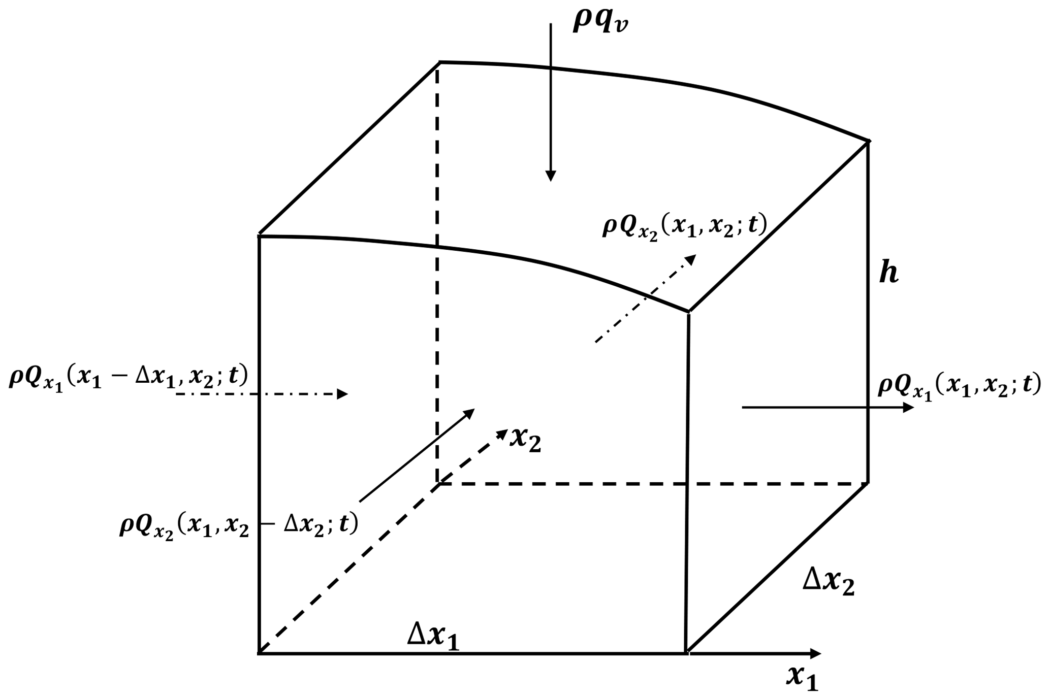
Under the Dupuit approximation of horizontal flow streamlines (for a very small water table gradient) (Bear, 1979), the net mass flux through the control volume of an unconfined aquifer with a flat bottom confining layer, as depicted in Fig. 1, which also has a sink/source mass flux, ρq_vΔx₁Δx₂, can be formulated as

\begin{matrix} (3) & \begin{aligned} [ρ Q_{x_{1}} (x_{1}, x_{2}; t) - ρ Q_{x_{1}} (x_{1} - Δ x_{1}, x_{2}; t)] Δ x_{2} \\ + [ρ Q_{x_{2}} (x_{1}, x_{2}; t) - ρ Q_{x_{2}} (x_{1}, x_{2} - Δ x_{2}; t)] Δ x_{1} \\ - ρ q_{v} Δ x_{1} Δ x_{2}, \end{aligned} \end{matrix}

where $Q_{x_{i}}$ is the discharge across a vertical plane of unit width in the ith direction (i=1, 2), ρ is the fluid density, and q_v is the source/sink (recharge/leakage) per unit horizontal area. Then, combining Eq. (2) with Eq. (3), with Δx_i=x_i (i=1, 2), and expressing the resulting Caputo derivative, $D_{0}^{β_{x_{i}}} f (x_{i})$ , as $\frac{\partial^{β_{x_{i}}} f (x_{i})}{{(\partial x_{i})}^{β_{x_{i}}}}$ (i=1, 2) for convenience, yields the net mass flux through the control volume in Fig. 1, to the orders of ${(Δ x_{1})}^{β_{x_{1}}}$ and ${(Δ x_{2})}^{β_{x_{2}}}$ , expressed as

\begin{matrix} (4) & \begin{aligned} \frac{1}{Γ (β_{x_{1}} + 1)} {(\frac{\partial}{\partial x_{1}})}^{β_{x_{1}}} (ρ Q_{x_{1}} (x_{1}, x_{2}; t)) {(Δ x_{1})}^{β_{x_{1}}} Δ x_{2} \\ + \frac{1}{Γ (β_{x_{2}} + 1)} {(\frac{\partial}{\partial x_{2}})}^{β_{x_{2}}} (ρ Q_{x_{2}} (x_{1}, x_{2}; t)) Δ x_{1} {(Δ x_{2})}^{β_{x_{2}}} \\ - ρ q_{v} Δ x_{1} Δ x_{2}, \end{aligned} \end{matrix}

where different powers for fractional space derivatives are utilized in different directions due to the anisotropy in the flow medium.

Kavvas et al. (2017b) have shown that, to $β_{x_{i}}$ -order fractional increments in space in the ith direction (i=1, 2),

\begin{matrix} (5) & {(Δ x_{i})}^{β_{x_{i}}} = \frac{Γ (β_{x_{i}} + 1) Γ (2 - β_{x_{i}})}{x_{i}^{1 - β_{x_{i}}}} Δ x_{i}, i = 1, 2 . \end{matrix}

Combining Eqs. (5) and (4) yields, for the net mass outflow through the control volume in Fig. 1 (to the orders of ${(Δ x_{i})}^{β_{x_{i}}}$ , i=1, 2),

\begin{matrix} (6) & \begin{aligned} \frac{Γ (2 - β_{x_{1}})}{x_{1}^{1 - β_{x_{1}}}} {(\frac{\partial}{\partial x_{1}})}^{β_{x_{1}}} (ρ Q_{x_{1}} (\overline{x}; t)) Δ x_{1} Δ x_{2} \\ + \frac{Γ (2 - β_{x_{2}})}{x_{2}^{1 - β_{x_{2}}}} {(\frac{\partial}{\partial x_{2}})}^{β_{x_{2}}} (ρ Q_{x_{2}} (\overline{x}; t)) Δ x_{1} Δ x_{2} \\ - ρ q_{v} Δ x_{1} Δ x_{2}, \overline{x} = (x_{1}, x_{2}) . \end{aligned} \end{matrix}

Denoting the water volume within the control volume in Fig. 1 by V_w, the specific yield (effective porosity) S_y of a phreatic aquifer (Bear and Verruijt, 1987) is expressed as

\begin{matrix} (7) & S_{y} = \frac{Δ V_{w}}{Δ h} \frac{1}{Δ x_{1} Δ x_{2}}, \end{matrix}

where ΔV_w is the change in water volume in the control volume per change Δh in the hydraulic head (the elevation of the phreatic surface (water table) above the flat bottom of the aquifer). The time rate of change in mass within the control volume in Fig. 1 may be written as (Bear and Verruijt, 1987)

\begin{matrix} (8) & \frac{S_{y} (ρ h (\overline{x}; t) - ρ h (\overline{x}; t - Δ t))}{Δ t} Δ x_{1} Δ x_{2}, \end{matrix}

which can then be expressed in terms of the approximation (Eq. 2) with respect to the time dimension as

\begin{matrix} (9) & \frac{S_{y}}{Δ t} [\frac{Δ t^{α}}{Γ (α + 1)} {(\frac{\partial}{\partial t})}^{α} (ρ h)] Δ x_{1} Δ x_{2} . \end{matrix}

To α-order fractional increments in time (Kavvas et al., 2017b)

\begin{matrix} (10) & {(Δ t)}^{α} = \frac{Γ (α + 1) Γ (2 - α)}{t^{1 - α}} Δ t . \end{matrix}

Substituting Eq. (10) into Eq. (9), one can obtain the time rate of change of mass in the control volume, as shown in Fig. 1,

\begin{matrix} (11) & S_{y} \frac{Γ (2 - α)}{t^{1 - α}} {(\frac{\partial}{\partial t})}^{α} (ρ h) Δ x_{1} Δ x_{2} . \end{matrix}

As the time rate of change of mass within the control volume, as shown in Fig. 1, must be inversely proportional to the net mass flux passing through the control volume, one may combine Eqs. (6) and (11) to obtain

\begin{matrix} (12) & \begin{aligned} [\frac{Γ (2 - β_{x_{1}})}{x_{1}^{1 - β_{x_{1}}}} {(\frac{\partial}{\partial x_{1}})}^{β_{x_{1}}} (ρ Q_{x_{1}} (\overline{x}; t)) \\ + \frac{Γ (2 - β_{x_{2}})}{x_{2}^{1 - β_{x_{2}}}} {(\frac{\partial}{\partial x_{2}})}^{β_{x_{2}}} (ρ Q_{x_{2}} (\overline{x}; t)) \\ - ρ q_{v}] Δ x_{1} Δ x_{2} = \\ - S_{y} \frac{Γ (2 - α)}{t^{1 - α}} {(\frac{\partial}{\partial t})}^{α} (ρ h) Δ x_{1} Δ x_{2}; \end{aligned} \\ (13) & \begin{aligned} \frac{Γ (2 - β_{x_{1}})}{x_{1}^{1 - β_{x_{1}}}} {(\frac{\partial}{\partial x_{1}})}^{β_{x_{1}}} (ρ Q_{x_{1}} (\overline{x}; t)) \\ + \frac{Γ (2 - β_{x_{2}})}{x_{2}^{1 - β_{x_{2}}}} {(\frac{\partial}{\partial x_{2}})}^{β_{x_{2}}} (ρ Q_{x_{2}} (\overline{x}; t)) - ρ q_{v} = \\ - S_{y} \frac{Γ (2 - α)}{t^{1 - α}} {(\frac{\partial}{\partial t})}^{α} (ρ h) \end{aligned} \end{matrix}

for $0 < α, β_{x_{1}}, β_{x_{2}} < 1$ , $\overline{x} = (x_{1}, x_{2},)$ .

Within the framework of fluid incompressibility in the unconfined aquifer, Eq. (13) reduces further to

\begin{matrix} (14) & \begin{aligned} \frac{Γ (2 - β_{x_{1}})}{Γ (2 - α)} \frac{t^{1 - α}}{x_{1}^{1 - β_{x_{1}}}} {(\frac{\partial}{\partial x_{1}})}^{β_{x_{1}}} (Q_{x_{1}} (\overline{x}; t)) \\ + \frac{Γ (2 - β_{x_{2}})}{Γ (2 - α)} \frac{t^{1 - α}}{x_{2}^{1 - β_{x_{2}}}} {(\frac{\partial}{\partial x_{2}})}^{β_{x_{2}}} (Q_{x_{2}} (\overline{x}; t)) \\ - \frac{t^{1 - α}}{Γ (2 - α)} q_{v} = - S_{y} \frac{\partial^{α} h}{{(\partial t)}^{α}}, \end{aligned} \end{matrix}

for $0 < α, β_{x_{1}}, β_{x_{2}} < 1$ , $\overline{x} = (x_{1}, x_{2},)$ , as the time–space fractional continuity equation of transient groundwater flow in an anisotropic unconfined aquifer with multi-fractional dimensions and in fractional time.

Performing a dimensional analysis of Eq. (14) yields

\begin{matrix} (15) & \begin{aligned} \frac{L}{T^{α}} & = \frac{T^{1 - α}}{L^{1 - β_{x_{1}}}} \frac{1}{L^{β_{x_{1}}}} \frac{L^{2}}{T} = \frac{T^{1 - α}}{L^{1 - β_{x_{2}}}} \frac{1}{L^{β_{x_{2}}}} \frac{L^{2}}{T} \\ = \frac{T^{1 - α}}{1} \frac{L}{T} = \frac{L}{T^{α}}, \end{aligned} \end{matrix}

where L denotes length and T denotes time. Also, α, $β_{x_{1}}$ , and $β_{x_{2}}$ are respectively the fractional powers in time and in x₁ and x₂ spatial dimensions. In Eq. (15), starting from the left-hand side (LHS), the first term shows the final dimensions of Eq. (14), the second term shows in detail the dimensions of the individual components of the first term on the LHS of Eq. (14), the third term shows in detail the dimensions of the individual components of the second term on the LHS of Eq. (14), the fourth term shows in detail the dimensions of the individual components of the third term on the LHS of Eq. (14), and the fifth term shows in detail the dimensions of the individual components on the right-hand side (RHS) of Eq. (14). Hence, the left-hand and right-hand sides of the continuity Eq. (14) for transient groundwater flow in an unconfined aquifer in multi-fractional space and fractional time are consistent, as shown in Eq. (15).

For $n - 1 < α, β_{x_{i}} < n$ , where n is any positive integer, as α and $β_{x_{i}} \to n$ , the Caputo fractional derivative of a function f(y) to order α or $β_{x_{i}}$ (i=1, 2) yields the standard nth derivative of the function f(y) (Podlubny, 1998). Then, when α and $β_{x_{i}} \to 1$ (i=1, 2), the continuity Eq. (14) becomes the conventional continuity equation for transient groundwater flow in an unconfined aquifer:

\begin{matrix} (16) & - S_{y} \frac{\partial h}{\partial t} = \frac{\partial}{\partial x_{1}} (Q_{x_{1}} (\overline{x}; t)) + \frac{\partial}{\partial x_{2}} (Q_{x_{2}} (\overline{x}; t)) - q_{v} . \end{matrix}

3 Motion equation (specific discharge equation) in fractional multidimensional unconfined aquifers

Recently, Kavvas et al. (2017a, b) derived a governing equation for water flux (specific discharge), $q_{x_{i}}$ (i=1, 2, 3), in a saturated or unsaturated porous medium with fractional dimensions in the form

\begin{matrix} (17) & \begin{aligned} q_{i} (\overline{x}, t) = - K_{s, x_{i}} (\overline{x}) \frac{Γ (2 - β_{x_{i}})}{x_{i}^{1 - β_{x_{i}}}} \frac{\partial^{β_{x_{i}}} h}{{(\partial x_{i})}^{β_{x_{i}}}}, \\ i = 1, 2, 3; \overline{x} = (x_{1}, x_{2}, x_{3}), \end{aligned} \end{matrix}

where $K_{s, x_{i}} (\overline{x})$ is the saturated hydraulic conductivity in the ith spatial direction (i=1, 2, 3). Meanwhile, under the Dupuit approximation of essentially horizontal unconfined aquifer flow (for a very small water table slope) (Bear, 1979), referring to Fig. 1, the discharge per unit width in the ith direction (i=1, 2) can be expressed as

\begin{matrix} (18) & Q_{x_{i}} (\overline{x}, t) = h q_{i} (\overline{x}, t), i = 1, 2; \overline{x} = (x_{1}, x_{2},) . \end{matrix}

Then combining Eqs. (18) and (17) results in

\begin{matrix} (19) & \begin{aligned} Q_{x_{i}} (\overline{x}, t) = - K_{s, x_{i}} (\overline{x}) \frac{Γ (2 - β_{x_{i}})}{x_{i}^{1 - β_{x_{i}}}} h \frac{\partial^{β_{x_{i}}} h}{{(\partial x_{i})}^{β_{x_{i}}}}, \\ i = 1, 2; \overline{x} = (x_{1}, x_{2}), \end{aligned} \end{matrix}

as the governing equation of groundwater motion within an unconfined aquifer with a flat bottom confining layer. In Eq. (19) h is the unconfined aquifer thickness or the phreatic surface elevation above the bottom confining layer.

A dimensional analysis of Eq. (19) yields L²∕T for the units of both the LHS and the RHS of the equation, establishing its dimensional consistency.

Applying the abovementioned result of Podlubny (1998) to the convergence of a fractional derivative to a corresponding integer derivative for $β_{x_{i}} \to 1$ (i=1, 2) reduces the fractional motion Eq. (19) for unconfined groundwater flow to the conventional equation (Bear, 1979):

\begin{matrix} (20) & Q_{x_{i}} (\overline{x}, t) = - K_{s, x_{i}} (\overline{x}) h \frac{\partial h (\overline{x}, t)}{\partial x_{i}}, i = 1, 2, \end{matrix}

for the case of integer spatial dimensions. As such, the fractional motion Eq. (19) for unconfined groundwater flow in fractional spatial dimensions is consistent with the conventional motion equation for the integer spatial dimensions.

4 The complete equation for transient unconfined groundwater flow in multi-fractional space and fractional time

Combining the fractional motion Eq. (19) of groundwater flow in an unconfined aquifer with the fractional continuity Eq. (14) of unconfined groundwater flow results in the equation

\begin{matrix} (21) & \begin{aligned} S_{y} \frac{\partial^{α} h}{{(\partial t)}^{α}} = \frac{Γ (2 - β_{x_{1}})}{x_{1}^{1 - β_{x_{1}}}} {(\frac{\partial}{\partial x_{1}})}^{β_{x_{1}}} \\ (K_{s, x_{1}} (\overline{x}) \frac{t^{1 - α}}{x_{1}^{1 - β_{x_{1}}}} \frac{Γ (2 - β_{x_{1}})}{Γ (2 - α)} h \frac{\partial^{β_{x_{1}}} h}{{(\partial x_{1})}^{β_{x_{1}}}}) \\ + \frac{Γ (2 - β_{x_{2}})}{x_{2}^{1 - β_{x_{2}}}} {(\frac{\partial}{\partial x_{2}})}^{β_{x_{2}}} \\ (K_{s, x_{2}} (\overline{x}) \frac{t^{1 - α}}{x_{2}^{1 - β_{x_{2}}}} \frac{Γ (2 - β_{x_{2}})}{Γ (2 - α)} h \frac{\partial^{β_{x_{2}}} h}{{(\partial x_{2})}^{β_{x_{2}}}}) \\ + \frac{t^{1 - α}}{Γ (2 - α)} q_{v}, \end{aligned} \end{matrix}

for $0 < α, β_{x_{1}}, β_{x_{2}} < 1$ , $\overline{x} = (x_{1}, x_{2},)$ , as the time–space fractional governing equation of transient unconfined groundwater flow in an anisotropic medium.

Performing a dimensional analysis of Eq. (21) yields

\begin{matrix} (22) & \begin{aligned} \frac{L}{T^{α}} & = \frac{1}{L^{1 - β_{x_{1}}}} \frac{1}{L^{β_{x_{1}}}} \frac{L}{T} \frac{T^{1 - α}}{L^{1 - β_{x_{1}}}} L \frac{L}{L^{β_{x_{1}}}} \\ = \frac{1}{L^{1 - β_{x_{2}}}} \frac{1}{L^{β_{x_{2}}}} \frac{L}{T} \frac{T^{1 - α}}{L^{1 - β_{x_{2}}}} \frac{L^{2}}{L^{β_{x_{2}}}} = \frac{T^{1 - α}}{1} \frac{L}{T} = \frac{L}{T^{α}}, \end{aligned} \end{matrix}

where L denotes length and T denotes time. Hence, the left-hand and right-hand sides of the governing Eq. (21) for transient groundwater flow in an unconfined aquifer in multi-fractional space and fractional time are consistent.

Specializing the above-discussed result of Podlubny (1998) to n=1, for α and $β_{x_{i}} \to 1$ (i=1, 2), reduces the governing fractional Eq. (21) to the conventional governing equation for transient groundwater flow in an unconfined aquifer (Bear, 1979):

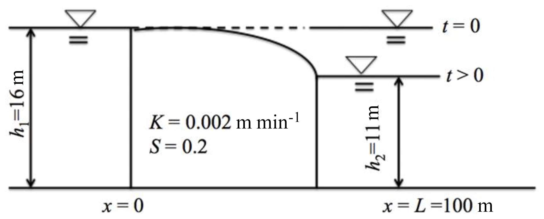
\begin{matrix} (23) & \begin{aligned} S_{y} \frac{\partial h}{\partial t} = \frac{\partial}{\partial x_{1}} (K_{s, x_{1}} (\overline{x}) h \frac{\partial h (\overline{x}, t)}{\partial x_{1}}) \\ + \frac{\partial}{\partial x_{2}} (K_{s, x_{2}} (\overline{x}) h \frac{\partial h (\overline{x}, t)}{\partial x_{2}}) + q_{v} . \end{aligned} \end{matrix}

https://www.earth-syst-dynam.net/11/1/2020/esd-11-1-2020-f02

Figure 2The sketch of numerical application 1; water seepage through the body of a dam as an unconfined groundwater flow.

Download

https://www.earth-syst-dynam.net/11/1/2020/esd-11-1-2020-f03

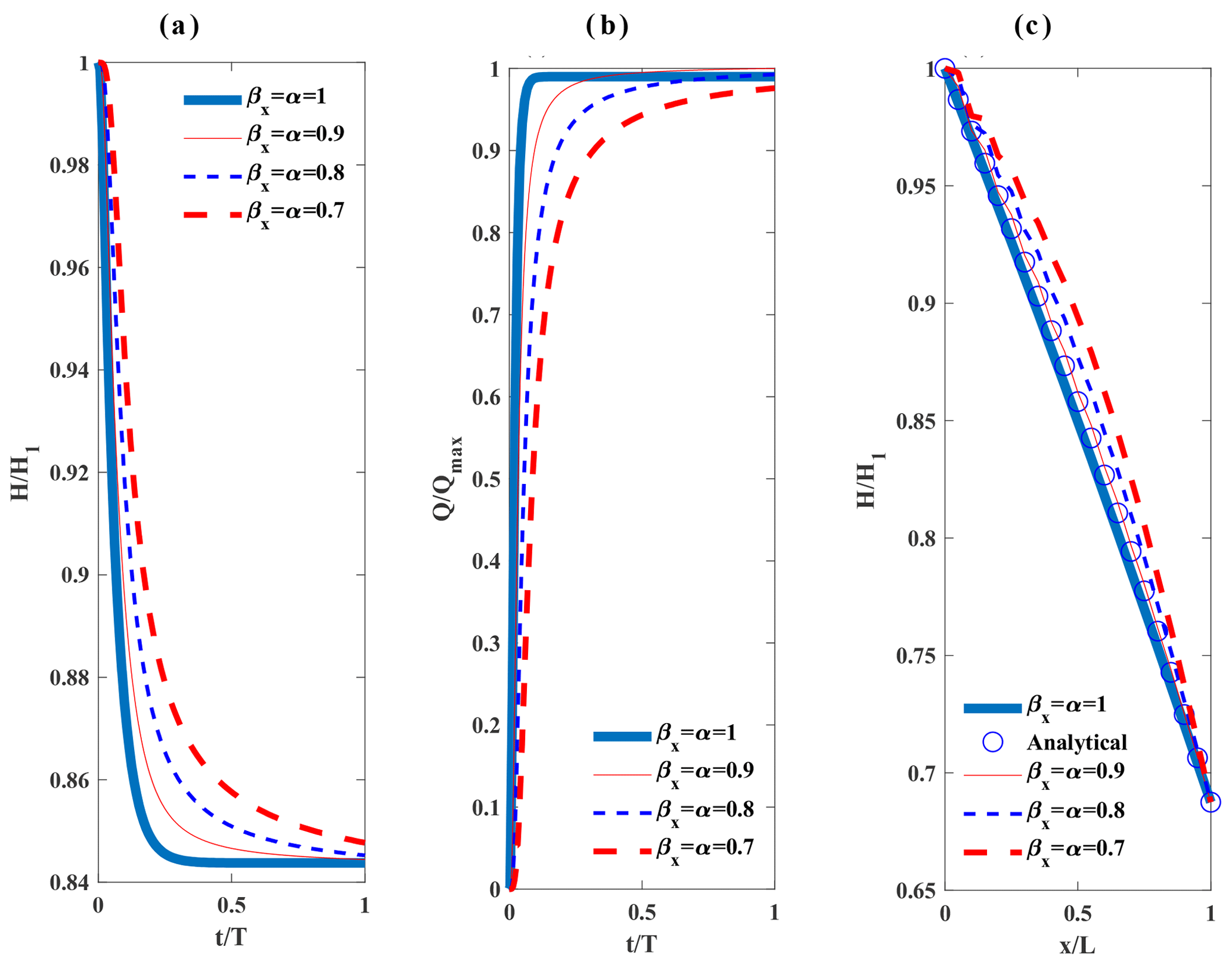
Figure 3Results for numerical application 1: (a) the normalized groundwater head at $x = L / 2$ through time under different fractional derivative powers; (b) the normalized groundwater discharge per unit width at $x = L / 2$ through time under different fractional derivative powers; t is time and the simulation time T is 120 000 min; (c) the normalized groundwater head at t=40 000 min through length of the aquifer (through the body of the dam) and the analytical solution to the conventional governing equation of unconfined groundwater flow when $β_{x} = α = 1$ at the steady state.

Download

5 Numerical application

To demonstrate the skills of the proposed fractional governing equation of unconfined aquifer groundwater flow, two numerical applications are performed using the proposed fractional governing equation. The first application (numerical application 1) follows the physical setting of an example from Wang and Anderson (1995), as depicted in Fig. 2. The numerical problem of seepage through a dam under a sudden change in the water surface elevation at the downstream section of the dam is modified based on seepage through a dam, p. 53 and Problem 4.4(a), p. 89 in Wang and Anderson (1995), as shown in Fig. 2. The water seepage through the body of the dam may be interpreted as one-dimensional groundwater flow through an unconfined aquifer. The unconfined flow system locates the top boundary of the saturated zone in an earthen dam and the bottom of the dam rests on impermeable rock. For this example, the unconfined aquifer length L is 100 m. The initial water level in the upstream and downstream sections of the dam and through the body of the dam is 16 m. Then immediately after the initial time, the water level at the downstream section of the dam is suddenly dropped to 11 m and remains at 11 m afterwards. The unconfined aquifer parameters are S=0.2 for the specific yield and K=0.002 m min⁻¹ for the hydraulic conductivity. The analytical solution to this problem at the steady state is

\begin{matrix} (24) & h = \sqrt{\frac{h_{2}^{2} - h_{1}^{2}}{L} x + h_{1}^{2}}, \end{matrix}

where h is the depth of the unconfined groundwater surface from the bottom layer, L is the aquifer length, x is the distance from the upstream location of the dam body, and h₁and h₂ are as shown in Fig. 2.

In Fig. 3a and b, the normalized groundwater head and normalized groundwater discharge per unit width at location $x = L / 2$ through time under different fractional power values are shown. Meanwhile, Fig. 3c shows the normalized groundwater head at the instance in time t=40 000 min as a function of location throughout the body of the dam and the analytical solution to the standard governing equation of unconfined groundwater flow when $β_{x} = α = 1$ at the steady state. The considered fractional derivative powers in space and time are $β_{x} = α = 0.7$ , 0.8, 0.9, 1.0. As can be seen from Fig. 3a, the hydraulic head recession in time slows down with the decrease of β_x=α from 1. The hydraulic heads in Fig. 3a have heavier tails as orders of time and space fractional derivative powers decrease from 1 towards 0.7. Furthermore, normalized groundwater discharge per unit width in Fig. 3b goes to 1 at a slower rate as fractional derivative powers decrease from 1 towards 0.7. Meanwhile, Fig. 3c shows that the numerical solution to the governing fractional equation at $β_{x} = α = 1.0$ and at a very long time after the initial condition perfectly matches the steady-state analytical solution, Eq. (24), to the standard Eq. (23) with the specified initial and boundary conditions.

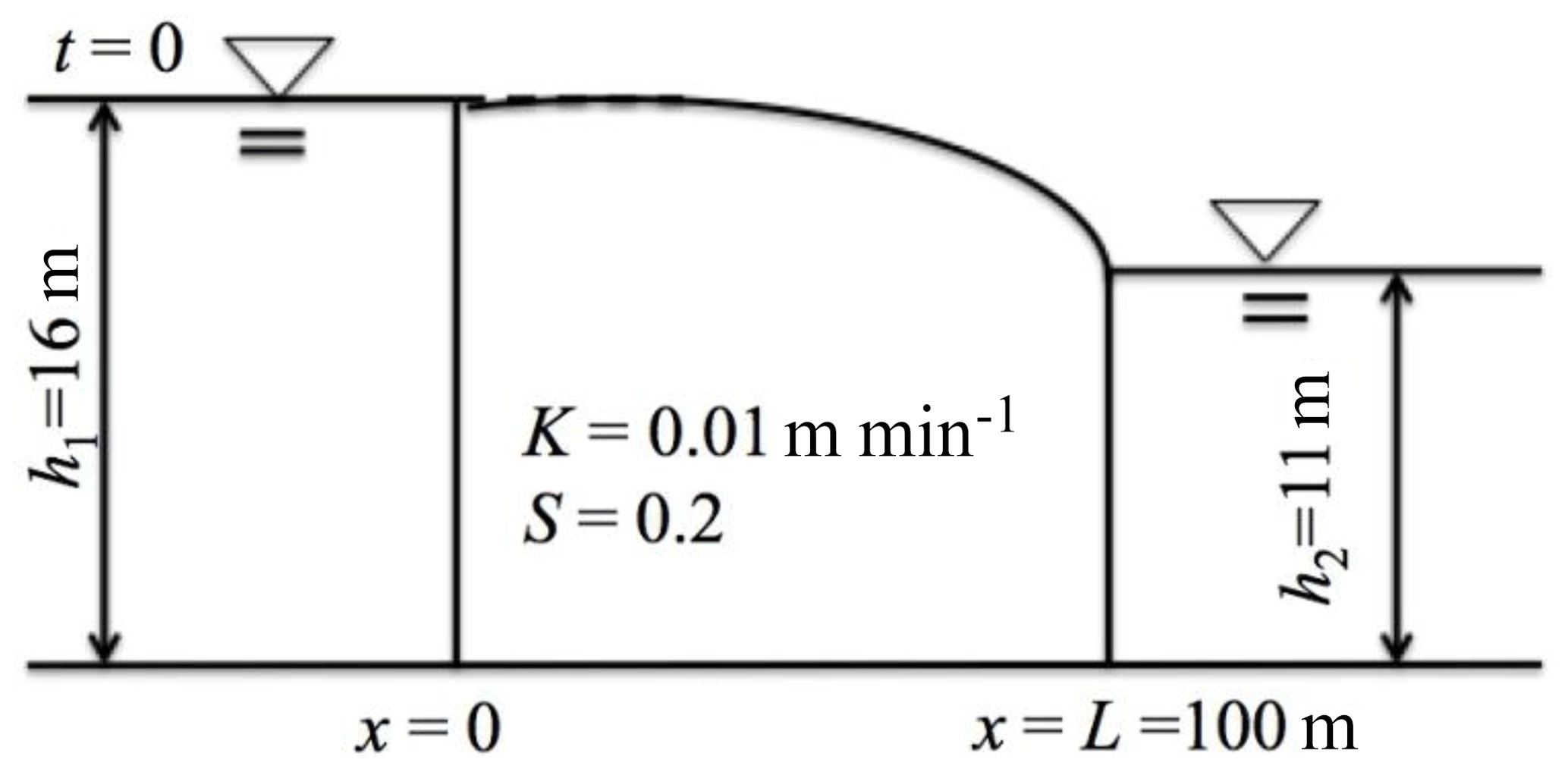
https://www.earth-syst-dynam.net/11/1/2020/esd-11-1-2020-f04

Figure 4The sketch numerical application 2; the downstream groundwater head is fixed at 11 m and the initial upstream groundwater head is 16 m.

Download

https://www.earth-syst-dynam.net/11/1/2020/esd-11-1-2020-f05

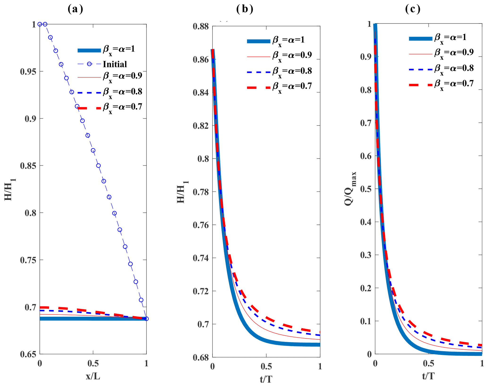
Figure 5Results for numerical application 2: (a) the normalized initial groundwater head in the unconfined aquifer and the normalized groundwater head at time t=60 000 min through length of the aquifer under different fractional derivative powers; (b) the normalized groundwater head at $x = L / 2$ through time under different fractional derivative powers; (c) the normalized groundwater discharge per unit width at $x = L / 2$ through time under different fractional derivative powers; t is time and the simulation time T is 60 000 min.

Download

The second application (numerical application 2) deals with a transient unconfined groundwater flow from a hillslope toward a stream (Fig. 4). The upstream boundary plane separates the region of flow from the adjacent hillslope that feeds the adjacent tributary system; therefore $\frac{\partial h}{\partial x} = 0$ (Freeze, 1978) at x=0. The normalized initial groundwater head in the unconfined aquifer and the normalized groundwater head at time t=60 000 min through the length of the aquifer under different fractional derivative powers are shown in Fig. 5a. The normalized groundwater head and normalized groundwater discharge per unit width at x=L/2 through time under different fractional derivative powers are demonstrated in Fig. 5b and c. As can be seen from Fig. 5b and c, the hydraulic head and groundwater discharge recession in time slows down with the decrease of β_x=α from 1. The hydraulic heads and groundwater discharges in Fig. 5b and c have heavier tails as orders of time and space fractional derivative powers decrease from 1 towards 0.7.

6 Discussion

From the standard governing Eq. (23) of unconfined groundwater flow in integer time–space the saturated hydraulic conductivity may be interpreted as a diffusion coefficient for the nonlinear diffusion of groundwater in an unconfined aquifer. The basic difference between confined and unconfined groundwater flow is that the former can be interpreted as a linear diffusion of groundwater while the latter is a nonlinear diffusion of groundwater within an aquifer. Similar to saturated hydraulic conductivities in Eq. (26) in Kavvas et al. (2017a) for the fractional confined aquifer groundwater flow, the saturated hydraulic conductivities in Eq. (21), which governs fractional unconfined aquifer groundwater flow, are modulated by the ratios of fractional time to fractional space, $\frac{t^{1 - α}}{x_{i}^{1 - β_{x_{i}}}}$ , i=1, 2. In other words, the confined and unconfined groundwater diffusions in fractional time–space are modulated by the above fractional time–space ratios.

Numerical applications demonstrated that as the powers of the space and time fractional derivatives decrease from 1, the recession rate of the nondimensional groundwater hydraulic head slows down compared to the case by the conventional governing equation (i.e., with integer-order derivatives). This behavior also indicates the modulation of the nonlinear diffusion of the groundwater by the fractional powers of time and space.

As mentioned in the Introduction section, unconfined groundwater flow is the fundamental component of the watershed runoff baseflow since it is the fundamental contributor to the streamflow network within a watershed during dry periods. As such, the behavior of unconfined groundwater flow is key to the physically based understanding of the long memory in watershed runoff. As seen from the numerical applications in Figs. 3 and 5, the powers of the fractional derivatives in time and space can modulate the speed of the groundwater discharge evolution. Hence, they can modulate the memory of the unconfined aquifer flow, which, in turn, can modulate the memory of the watershed baseflow. Meanwhile, the Caputo derivative, as defined in its special form $D_{0}^{β_{x_{i}}} f (x_{i})$ in space in this study, was shown by Kavvas and Ercan (2016) and Ercan and Kavvas (2017) to be a nonlocal quantity where the effect of the boundary conditions on the groundwater flow within the flow domain can have long spatial memories with the decrease in the powers of the spatial fractional derivatives from unity. Similarly, it was shown by Kavvas et al. (2017a) that the Caputo derivative in time, $D_{0}^{α} f (t)$ , as defined in this study, is nonlocal in time and can carry the effect of initial conditions on the groundwater flow for long time periods as the power in the time fractional derivative decreases from 1. Therefore, the fractional governing equation of unconfined groundwater flow in fractional time and multi-fractional space has the potential to describe the long-memory characteristics of baseflow within a watershed. This important topic shall be explored in the near future.

7 Conclusion

A dimensionally consistent fractional governing equation of transient unconfined aquifer groundwater flow was derived within a fractional differentiation framework. After developing a fractional continuity equation, a previously developed dimensionally consistent equation for water flux in unsaturated/saturated porous media was combined with the Dupuit approximation to obtain an equation for groundwater motion in multi-fractional space in unconfined aquifers. By combining the fractional continuity and motion equations, the governing equation of transient unconfined aquifer groundwater flow in a multi-fractional medium in fractional time was obtained. To demonstrate the skills of the proposed fractional governing equation of unconfined aquifer groundwater flow, two numerical applications were performed. As demonstrated in the numerical application results, the orders of the fractional space and time derivatives modulate the speed of groundwater discharge and groundwater flow evolution, slowing the process with the decrease in the powers of the fractional derivatives from 1. It is also shown that the proposed dimensionally consistent fractional governing equations approach the corresponding conventional equations as the fractional orders of the derivatives go to 1.

Data availability

The data used in this article can be accessed by contacting the corresponding author.

Appendix A: Numerical solution for the one-dimensional case

One-dimensional time–space fractional groundwater flow in the unconfined aquifer with no recharge or leakage can be written as

\begin{matrix} (A1) & \begin{aligned} S_{y} \frac{\partial^{α} h}{{(\partial t)}^{α}} = \frac{Γ (2 - β)}{x^{1 - β}} {(\frac{\partial}{\partial x})}^{β} \\ (K_{s} (\overline{X}) \frac{t^{1 - α}}{x^{1 - β}} \frac{Γ (2 - β)}{Γ (2 - α)} h \frac{\partial^{β} h}{{(\partial x)}^{β}}) . \end{aligned} \end{matrix}

The fractional time and space derivatives are estimated in the same manner as seen in Tu et al. (2018), where the Caputo fractional space and time derivatives in the fractional governing equation are estimated by the numerical algorithm in Odibat (2009) and the algorithm reported by Murio (2008), respectively. The Caputo fractional space derivative ${D_{x}^{β} f (x)|}_{x = L} {D_{x}^{β} g (x)|}_{x = L}$ at the location L for $m - 1 < β \leq m$ (m∈N) for a given space interval [0,L] is estimated as

\begin{matrix} (A2) & \begin{aligned} {D_{x}^{β} g (x)|}_{x = L} \approx \frac{Δ L^{m - β}}{Γ (m + 2 - β)} {[{(N - 1)}^{m - β + 1} \\ - (N - m + β - 1) Δ L^{m - β}] g^{(m)} (0) + g^{(m)} (L) \\ + \sum_{i = 1}^{N - 1} [{(N - i + 1)}^{m - β + 1} - 2 {(N - i)}^{m - β + 1} \\ + {(N - i - 1)}^{m - β + 1}] g^{(m)} (l_{i})}, \end{aligned} \end{matrix}

where N is the number of equally spaced subintervals on [0,L]; the subinterval length is $Δ L = L / N$ and l_i=iΔL, for $i = 0, 1, 2, \dots, N$ .

The Caputo fractional time derivative ${D_{t}^{α} g (x, t)|}_{x = l_{i}, t = t_{n}}$ for $0 < α \leq 1$ for a given time interval [0,T], which is divided into M equal subintervals with a time window of $Δ t = T / M$ by using the nodes t_n=nΔt, $n = 0, 1, 2, \dots, M$ , can be approximated as

\begin{matrix} (A3) & \begin{aligned} D_{t}^{α} g_{i}^{n} = \frac{Δ t^{- α}}{Γ (2 - α)} \sum_{k = 1}^{n} [k^{1 - α} - {(k - 1)}^{1 - α}] \\ (g_{i}^{n - k + 1} - g_{i}^{n - k}) . \end{aligned} \end{matrix}

Then the 1-D governing equation in fractional time and space for Cartesian groundwater flow in an unconfined aquifer can be discretized as

for n=1,
$\begin{matrix} (A4) & h_{i}^{n} = h_{i}^{n - 1} + \frac{t_{n}^{1 - α}}{S_{y} Δ t^{- α}} \frac{Γ (2 - β)}{l_{i}^{1 - β}} G_{i}^{n - 1} . \end{matrix}$
for n≥2,
$\begin{matrix} (A5) & \begin{aligned} h_{i}^{n} = h_{i}^{n - 1} + \frac{t_{n}^{1 - α}}{S_{y} Δ t^{- α}} \frac{Γ (2 - β)}{l_{i}^{1 - β}} G_{i}^{n - 1} \\ - \sum_{k = 2}^{n} [k^{1 - α} - {(k - 1)}^{1 - α}] (h_{i}^{n - k + 1} - h_{i}^{n - k}), \end{aligned} \end{matrix}$

where $G = {(\frac{\partial}{\partial x})}^{β} [K_{s} (\overline{X}) \frac{Γ (2 - β)}{x^{1 - β}} h \frac{\partial^{β} h}{\partial x^{β}}]$ , and the space and time fractional derivatives in G are estimated as in Eqs. (A2) and (A3).

Author contributions

MLK wrote the main body of the paper. TT and AE wrote the numerical applications section. MLK, TT, AE, and JP discussed the results and responded to the reviewers.

Competing interests

The authors declare that they have no conflict of interest.

Acknowledgements

Authors thank the editor Rui A. P. Perdigão and two anonymous referees for their valuable comments and suggestions.

Review statement

This paper was edited by Rui A. P. Perdigão and reviewed by two anonymous referees.

References

Atangana, A.: Drawdown in prolate spheroidal–spherical coordinates obtained via Green's function and perturbation methods, Commun. Nonlinear Sci., 19, 1259–1269, 2014.

Atangana, A. and Baleanu, D.: Modelling the advancement of the impurities and the melted oxygen concentration within the scope of fractional calculus, Int. J. Nonlin. Mech., 67, 278–284, 2014.

Atangana, A. and Bildik, N.: The use of fractional order derivative to predict the groundwater flow, Math. Probl. Eng., 2013, 543026, https://doi.org/10.1155/2013/543026, 2013.

Atangana, A. and Vermeulen, P.: Analytical solutions of a space-time fractional derivative of groundwater flow equation, Abstr. Appl. Anal., 2014, 381753, https://doi.org/10.1155/2014/381753, 2014.

Bear, J.: Groundwater hydraulics, McGraw, New York, USA, 1979.

Bear, J. and Verruijt, A.: Modeling Groundwater Flow and Pollution, Reidel Pub. Co., Dordrecht, the Netherlands, 1987.

Beran, J.: Statistics for Long-Memory Processes, in: Monographs on Statistics and Applied Probability, vol. 61, Chapman & Hall, New York, USA, 1994.

Black, J. H., Barker, J. A., and Noy, D. J.: Crosshole investigations-the method, theory and analysis of crosshole sinusoidal pressure tests in fissured rock, Stripa Projects Internal Reports 86-03, SKB, Stockholm, Sweden, 1986.

Cloot, A. and Botha, J.: A generalised groundwater flow equation using the concept of non-integer order derivatives, Water SA, 32, 1–7, 2006.

Diethelm, K.: The mean value theorems and a Nagumo-type uniqueness theorem for Caputo's fractional calculus, Fract. Calc. Appl. Anal., 15, 304–313, https://doi.org/10.2478/s13540-012-0022-3, 2012.

Eltahir, E. A. B.: El Nino and the natural variability in the flow of the Nile River, Water Resour. Res., 32, 131–137, 1996.

Ercan, A. and Kavvas, M. L.: Time–space fractional governing equations of one-dimensional unsteady open channel flow process: Numerical solution and exploration, Hydrol. Process., 31, 2961–2971, 2017.

Freeze, R. A.: Mathematical models of hillslope hydrology, in: Hillslope Hydrology, chap. 6, edited by: Kirkby, M. J., John Wiley & Sons, Ltd, New York, USA, 1978.

Freeze, R. A. and Cherry, J. A.: Groundwater, Prentice-Hall, Englewood Cliffs, NJ, USA, 1979.

Hurst, H. E., Long term storage capacities of reservoirs, T. Am. Soc. Civ. Eng., 116, 776–808, 1951.

Kavvas, M. L. and Ercan, A.: Time-Space Fractional Governing Equations of Unsteady Open Channel Flow, J. Hydrol. Eng., 22, 04016052, https://doi.org/10.1061/(ASCE)HE.1943-5584.0001460, 2016.

Kavvas, M. L., Tu, T., Ercan, A., and Polsinelli, J.: Fractional governing equations of transient groundwater flow in confined aquifers with multi-fractional dimensions in fractional time, Earth Syst. Dynam., 8, 921–929, https://doi.org/10.5194/esd-8-921-2017, 2017a.

Kavvas, M. L., Ercan, A., and Polsinelli, J.: Governing equations of transient soil water flow and soil water flux in multi-dimensional fractional anisotropic media and fractional time, Hydrol. Earth Syst. Sci., 21, 1547–1557, https://doi.org/10.5194/hess-21-1547-2017, 2017b.

Khalil, R., Al Horani, M., Yousef, A., and Sababheh, M.: A new definition of fractional derivative, J. Comput. Appl. Math., 264, 65–70, 2014.

Klemes, V.: The Hurst phenomenon: a puzzle?, Water Resour. Res., 10, 675–688, 1974.

Koutsoyiannis, D.: The Hurst phenomenon and fractional Gaussian noise made easy, Hydrolog. Sci. J., 47, 573–595, 2002.

Koutsoyiannis, D.: Climate change, the Hurst phenomenon, and hydrological statistics, Hydrolog. Sci. J., 48, 3–24, 2003.

Koutsoyiannis, D.: Hydrologic Persistence and The Hurst Phenomenon, in: The Encylopedia of Water, chap. 5, https://doi.org/10.1002/047147844X.sw434, 2005.

Li, M.-F., Ren, J.-R., and Zhu, T.: Series expansion in fractional calculus and fractional differential equations, arXiv preprint arXiv:0910.4819, available at: https://arxiv.org/pdf/0910.4819.pdf (last access: 15 December 2019), 2009.

Li, Z. and Zhang, Y.-K.: Quantifying fractal dynamics of groundwater systems with detrended fluctuation analysis, J. Hydrol., 336, 139–146, 2007.

Mandelbrot, B. B.: The Fractal Geometry of Nature, Freeman, New York, USA, 1977.

Mandelbrot, B. B. and Wallis, J. R.: Computer experiments with fractional Gaussian noises, Part 2: Rescaled ranges and spectra, Water Resour. Res., 5, 242–259, 1969.

Mehdinejadiani, B., Jafari, H., and Baleanu, D.: Derivation of a fractional Boussinesq equation for modelling unconfined groundwater, Eur. Phys. J. Spec. Top., 222, 1805–1812, https://doi.org/10.1140/epjst/e2013-01965-1, 2013.

Montanari, A., Rosso, R., and Taqqu, M. S.: Fractionally differenced ARIMA models applied to hydrologic time series, Water Resour. Res., 33, 1035–1044, 1997.

Murio, D. A.: Implicit finite difference approximation for time fractional diffusion equations, Comput. Math. Appl., 56, 1138–1145, 2008.

Odibat, Z. M.: Computational algorithms for computing the fractional derivatives of functions, Math. Comput. Simulat., 79, 2013–2020, 2009.

Odibat, Z. M. and Shawagfeh, N. T.: Generalized Taylor's formula, Appl. Math. Comput., 186, 286–293, 2007.

Olsen, J. S., Mortensen, J., and Telyakovskiy, A. S.: A two-sided fractional conservation of mass equation, Adv. Water Resour., 91, 117–121, https://doi.org/10.1016/j.advwatres.2016.03.007, 2016.

Podlubny, I.: Fractional differential equations: an introduction to fractional derivatives, fractional differential equations, to methods of their solution and some of their applications, Academic press, San Diego, CA, USA, 1998.

Radziejewski, M. and Kundzewicz, Z. W., Fractal analysis of flow of the river Warta, J. Hydrol., 200, 280–294, 1997.

Su, N.: The fractional Boussinesq equation of groundwater flow and its applications, J. Hydrol., 547, 403–412, https://doi.org/10.1016/j.jhydrol.2017.01.015, 2017.

Tu, T., Ercan, A., and Kavvas, M. L.: Fractal scaling analysis of groundwater dynamics in confined aquifers, Earth Syst. Dynam., 8, 931–949, https://doi.org/10.5194/esd-8-931-2017, 2017.

Tu, T., Ercan, A., and Kavvas, M. L.: Time–space fractional governing equations of transient groundwater flow in confined aquifers: Numerical investigation, Hydrol. Process., 32, 1406–1419, 2018.

Usero, D.: Fractional Taylor series for Caputo fractional derivatives. Construction of numerical schemes, available at: https://www.semanticscholar.org/paper/Fractional-Taylor-Series-for-Caputo-Fractional-of-Usero/4d99ce0c656857f8ca764d3914cd601c86d44969 (last access: 15 December 2019), 2008.

Van Tonder, G., Botha, J., Chiang, W.-H., Kunstmann, H., and Xu, Y.: Estimation of the sustainable yields of boreholes in fractured rock formations, J. Hydrol., 241, 70–90, 2001.

Vogel, R. M., Tsai, Y., and Limbrunner, J. F.: The regional persistence and variability of annual streamflow in the United States, Water Resour. Res., 34, 3445–3459, 1998.

Wang, H. F. and Anderson, M. P.: Introduction to groundwater modeling: finite difference and finite element methods, Academic Press, San Diego, CA, USA, 1995.

Wheatcraft, S. W. and Meerschaert, M. M.: Fractional conservation of mass, Adv. Water Resourc., 31, 1377–1381, 2008.

Yevjevich, V.: Fluctuations of wet and dry years: Part 1: Research data assembly and mathematical models, Hydrology Papers, Colorado State University, Ft. Collins, Colorado, USA, 1963.

Yevjevich, V.: Stochastic Processes in Hydrology, Wat. Resour. Pub., Ft. Collins, Colorado, USA, 1971.

Yu, X., Ghasemizadeh, R., Padilla, I. Y., Kaeli, D., and Alshawabkeh, A.: Patterns of temporal scaling of groundwater level fluctuation, J. Hydrol., 536, 485–495, 2016.