the Creative Commons Attribution 4.0 License.
the Creative Commons Attribution 4.0 License.
 | 30 Jul 2019
Downslope windstorms in the Isthmus of Tehuantepec during Tehuantepecer events: a numerical study with WRF high-resolution simulations
Miguel A. Prósper
Ian Sosa Tinoco
Carlos Otero-Casal
Gonzalo Miguez-Macho
Tehuantepecers or Tehuanos are extreme winds produced in the Isthmus of Tehuantepec, blowing south through Chivela Pass, the mountain gap across the isthmus, from the Gulf of Mexico into the Pacific Ocean. They are the result of the complex interaction between large-scale meteorological conditions and local orographic forcings around Chivela Pass, and occur mainly in winter months due to cold air damming in the wake of cold fronts that reach as far south as the Bay of Campeche. Even though the name refers mostly to the intense mountain gap outflow, Tehuantepecer episodes can also generate other localized extreme wind conditions across the region, such as downslope windstorms and hydraulic jumps, which are strong turbulent flows that have a direct effect on the Pacific side of the isthmus and the Gulf of Tehuantepec.
This study focuses on investigating these phenomena using high horizontal and vertical resolution WRF (Weather Research and Forecasting) model simulations. In particular, we employ a 4-nested grid configuration with up to 444 m horizontal spacing in the innermost domain and 70 hybrid-sigma vertical levels, 8 of which lie within the first 200 m above ground. We select one 36 h period in December 2013, when favorable conditions for a strong gap wind situation were observed. The high-resolution WRF experiment reveals a significant fine-scale structure in the strong Tehuano wind flow, beyond the well known gap jet. Depending on the Froude number upstream of the topographic barrier, different downslope windstorm conditions and hydraulic jumps with rotor circulations develop simultaneously at different locations east of Chivela Pass with varied crest height. A comparison with observations suggests that the model accurately represents the spatially heterogeneous intense downslope windstorm and the formation of mountain wave clouds for several hours, with low errors in wind speed, wind direction and temperature.
- Article
(5505 KB) -
Supplement
(223299 KB) - BibTeX
- EndNote


The Isthmus of Tehuantepec, in the Mexican state of Oaxaca, is the narrowest stretch of land separating the Gulf of Mexico from the Pacific Ocean. The Sierra Madre mountains cross the isthmus from east to west, but leaving a pronounced gap in the middle (Chivela Pass), coinciding with the point of shortest distance between the two sea masses of only 200 km. The elevation of the Chivela Pass is 224 m, whereas mountain peaks in the side sierras reach 2000 m, creating ideal conditions to generate a powerful wind corridor (Romero-Centeno et al., 2003). In winter, cold high-pressure systems originating in North America move over the Gulf of Mexico in the wake of south-reaching cold fronts, and large pressure differences develop across the isthmus between the Bay of Campeche and the Gulf of Tehuantepec, on the Pacific side. This pressure gradient results in a northerly wind situation in which the flow is accelerated southward by cold air damming, traveling through Chivela Pass to finally blow violently outward into the Pacific Ocean as it fans out and curves anticyclonically. This gap outflow extends for hundreds of kilometers over the Gulf of Tehuantepec, a result of the combined effect of the open marine surface and the low Coriolis parameter of the tropical latitude of the area. The small impact of planetary rotation yields very weak synoptic forcing; thus, the gap wind does not encounter any ambient large-scale flow to merge with, describing a very-close-to-inertial trajectory with a large radius, also as a consequence of the diminished Coriolis force (Steenburgh et al., 1998). In the Gulf of Tehuantepec, the strong sea surface wind stress generates intense upwelling and vertical mixing in the upper ocean (Hong et al., 2018). The largest number of these events tends to occur in December, with a mean duration of 48 h (Brennan et al., 2010). These powerful mountain gap winds are called Tehuantepecers or Tehuanos and have been the focus of several previous studies (Brennan et al., 2010; McCreary et al., 1989; Jaramillo and Borja, 2004) detailing their general setting, drivers and dynamics (Steenburgh et al., 1998) of strong wind situations in the isthmus. Little knowledge exists, however, on the fine-scale structure of the Tehuantepecer flow elsewhere across the isthmus, away from Chivela Pass. There is evidence from observations and earlier numerical studies (Steenburgh et al., 1998) that the low-elevation topography of Chivela Pass can excite mountain waves and also that these are not only restricted to the pass itself but extend into the much higher mountain crests to the west and especially to the east, as the cold air pool is often thick enough to surpass them. This gravity wave activity can potentially result in downslope windstorms (DSWSs hereafter) producing severe turbulent phenomena such as rotors and hydraulic jumps (HJs hereafter) (Durran, 1986a; Sheridan and Vosper, 2006) on the Pacific side of the isthmus, to the lee of local orography, which would explain several accidents related to strong winds reported by the Oaxaca's Civil Protection Commission (Santiago, 2018; Hernández, 2018; Televisa, 2018; Rodríguez, 2018) every year during some Tehuano occurrences. The ability to understand and forecast these events is very relevant since the isthmus has been an important development site for wind farms since the 2000s (Coldwell et al., 2017). Currently this region allocates 76.8 % of the wind power capacity installed in Mexico, with approximately 2360 MW (Baxter et al., 2017), which is expected to double to 5076 MW by 2020 (Francisco Ibáñez, 2018).
The main goal of the present work is to study the variability in flow behavior, beyond the well-known mountain gap jet, in Tehuano wind episodes across the Isthmus of Tehuantepec, depending on topographic barrier height and thermodynamic conditions of the air mass, using high-resolution simulations with the Weather Research and Forecasting (WRF) model. Many studies have successfully employed WRF to analyze these kinds of mountain-flow events in other parts of the world. In the US, for example, Pokharel et al. (2017b) study a DSWS and HJ to the lee of the Medicine Bow Mountains in southeast Wyoming. Another DSWS in this same area is also investigated by Grubišić et al. (2015) with WRF. Other studies such as Cao and Fovell (2016), Pokharel et al. (2017a), Prtenjak and Belusic (2009), Jung-Hoon and Chung (2006), Ágústsson and Ólafsson (2014), and Priestley et al. (2017) also use WRF at high resolution to analyze mountain wave flows in different locations. To the best of our knowledge, there is no previous work that studies in detail lee wave phenomena in the Mexican state of Oaxaca.
The high-resolution WRF simulations employed in the present study allow us to obtain a more complete knowledge of these events, from the synoptic scale to the small scale, focusing on the downslope winds and the HJ that develop along the mountain ranges neighboring Chivela Pass. The article is organized as follows: in Sect. 2 the methodology is explained in detail, from the climatology of the region to the model configuration. In Sect. 3, the primary results obtained are shown, divided into synoptic-mesoscale situations and the upstream–downstream structure of the phenomena. Finally, in Sect. 4 the conclusions reached are discussed.
1.1 Mountain wave phenomena, hydraulic analog and relation with the Froude number
DSWSs result from the intense flow acceleration occurring on the lee slope of a mountain under certain cross-barrier wind conditions. They resemble the behavior of water flow in an open channel when encountering an obstacle, such as when a relatively slow river increases its speed when flowing in a thin layer over a mill's dam or over a rock. As in the case of the river, DSWSs often end abruptly with a return to the state upstream of the obstacle through a turbulent HJ somewhere downstream. The similarity in both fluid's behavior suggests that the physical processes behind them are also alike, and that shallow-water theory could be applied somehow to the atmosphere (Long, 1953). However, the complexity of the unbounded atmospheric flow, without a free surface, makes it difficult to make the analog so simple because gravity waves in the atmosphere propagate vertically in addition to horizontally as in shallow water, and nonlinear effects are important.
Considerable observational and numerical experiments have been developed to elucidate the dynamics of atmospheric mountain lee flows (see Durran, 1990, for a review). The current view is that in the atmosphere DSWSs are observed when stable air at low levels flows, similarly to shallow water, as if having a free surface somewhere above the obstacle preventing vertical energy dissipation. This occurs when gravity waves do not propagate vertically and break because of the presence of a critical level (Durran and Klemp, 1987) or due to overturning for having an amplitude that is too large (Clark and Peltier, 1977), or when without wave breaking there is an interface separating highly stable lower layers from less-stable air above (Durran, 1986b; Klemp and Durran, 1987; Bacmeister and Pierrehumbert, 1988). Wave breaking creates a well-mixed layer to the lee of the obstacle, which generates a dividing streamline separating undisturbed flow aloft and trapped energy and flow analogous to hydraulics in the lower surficial branch (Smith, 1985b). A highly stable lower layer topped by less-stable air results in reflecting and decaying waves aloft, enhanced nonlinear effects, and the atmosphere also flowing like a two-layer fluid and behaving like shallow water when encountering the barrier.
In shallow water theory, the Froude number (Fr), which is the ratio of the mean speed to the intrinsic gravity wave phase speed in the fluid, determines its behavior when encountering the obstacle, depending on whether gravity is balanced mostly by acceleration (Fr>1) or pressure gradient forces (Fr<1). HJs and significant flow acceleration to the lee of the obstacle occur when the fluid transitions from a subcritical (Fr<1) to supercritical (Fr>1) regime at the top of the barrier. It is not straightforward to define a Froude number to determine the regime of atmospheric flows (Sheridan and Vosper, 2006; Smith, 1989, 1985a) as it is for shallow water because there is no clear analog to flow depth controlling gravity wave speed and pressure perturbations. Key factors determining wave properties and flow characteristics in this case are stratification, wind speed and barrier height, or rather the relative values among them. A quantity that combines these three variables, and is referred to as Froude number for shallow atmospheric flows over mountains by many authors, is the following (Smith, 1989):
where U is the flow speed, N the Brunt–Väisäla frequency (Eq. 2) and H the mountain height.
with g being the acceleration due to gravity, dθ∕dt the potential temperature gradient in the stable layer and θ0 the potential temperature at the base of this layer. To avoid confusion with the classical Froude number, the inverse of Fr defined as above is often used instead and called the nondimensional mountain height. Fr is a measure of flow deceleration and stagnation upwind from the mountain (Baines, 1987). It can also be regarded as an estimate of nonlinearity. When Fr≪1 there are significant nonlinear effects and blocking, whereas for Fr≫1 the opposite occurs (Smolarkiewicz and Rotunno, 1989). Fr around 1 indicates a transitional regime between the two states and favorable conditions for the formation of DSWS and HJs.
2.1 WRF configuration
We use the Advanced Research WRF (ARW) model (Skamarock et al., 2008) version 3.9 (WRFV3.9) to perform the simulations. Based on a fully compressible and nonhydrostatic dynamic core, WRFV3.9 is a limited-area mesoscale and microscale model, with a terrain-following hydrostatic-pressure vertical coordinate designed for operational forecasting, as well as research. For the experiments, we employ a nested domain configuration in order to achieve sufficiently high resolution in the innermost grids to capture the small-scale structure of the flow, while reproducing the synoptic phenomenology conducive to local DSWS in the parent one (Fig. 1a).
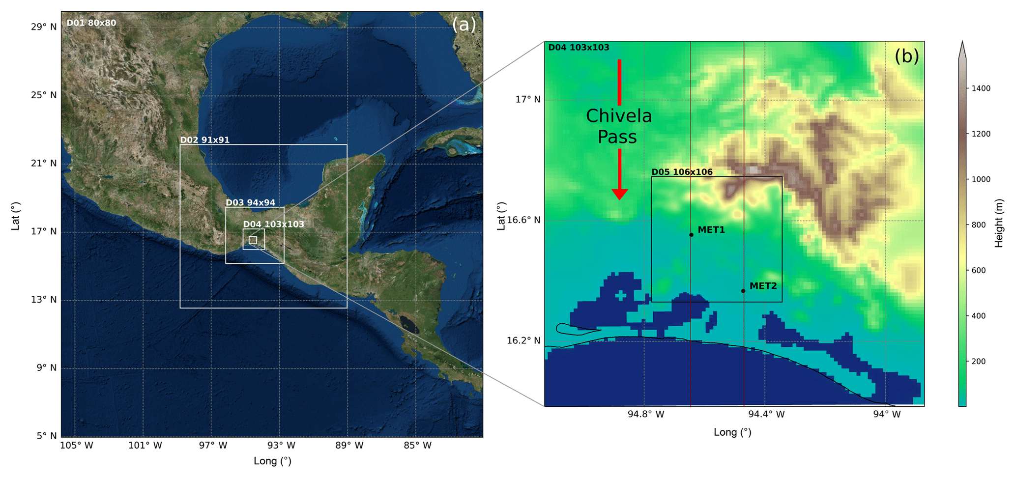
Figure 1WRF nested domain configuration. (a) Coarser three domains with their number of grid points. (b) Higher-resolution domains (d04 and d05), both with their respective topographies (meters above sea level). MET1 and MET2 are the locations of the meteorological stations used as validation points. The two red lines represent the vertical cross sections shown in Figs. 3 and 5.
The domain's configuration meets the requirements recommended by Warner (2011), including a parent (d01) and four nested grids (d02, d03, d04 and d05) (Fig. 1a) that are one-way interacting. D01 is centered at 17.91∘ N, 93.44∘ W (Fig. 1a) with 80×80 grid points of 36 km of horizontal resolution. The horizontal resolutions of d02–d05 are 12 km (91×91 grid points), 4 km (94×94 grid points), 1.3 km (103×103 grid points) and 444 m (106×106 grid points) respectively. D03 covers the whole isthmus area, with Chivela Pass approximately at its center, while the highest resolution domains, d04 and d05, are slightly displaced to the south and east, respectively. D04 includes Chivela Pass and the section of the Sierra Madre de Chiapas range east of it, with heights reaching about 2000 m. For its part, the finest grid D05 encompasses the southernmost hills to the east of Chivela Pass and the coastal plain at their base. This domain configuration focuses the area of interest of the study on the Pacific side of the Tehuano, encompassing the flow path before and after crossing the mountains, the exit section of the mountain gap and the gradually rising mountains east of it, around the only two available observational sites for validation, labeled as MET1 and MET2 in Fig. 1b.
All the domains have 70 hybrid-sigma vertical levels, 8 of which lie within the first 200 m above ground at about 16, 46, 71, 96, 122, 147, 173 and 198 m heights. The hybrid sigma-pressure vertical coordinate follows the terrain near the surface and gradually transitions to constant pressure at higher levels. The benefit of this vertical coordinate system is a numerical noise reduction in the upper layers over mountains (Powers et al., 2017). We maintain this fine vertical grid spacing in all the domains to capture as wide a range of motions as possible over the depth of the boundary layer.
Land use information for d04 and d05 is obtained from the ESA CCI (European Space Agency Climate Change Initiative) database (Bontemps et al., 2013) with a resolution of 300 m. The terrain elevation used comes from the ASTER Global Digital Elevation Map (GDEM) from USGS (United States Geological Survey) (Slater et al., 2009) with a resolution of 30 m. In the other domains, terrain and land use data are from the WRF global standard database, both at 30 arcsec resolution for d03 and 2 arcmin for d02 and d01.
We simulate a 36 h period, from 23 December 12:00 to 25 December 2013 00:00 UTC, which registers DSWS conditions in the observational data. Regarding the main physics options, the simulations use the tropical suite configuration (Table 1), introduced in WRF version 3.9, except for the planetary boundary layer, which is parametrized by the Shin–Hong scale-aware scheme (S–H) (Shin and Hong, 2015). Table 1 summarizes this physics configuration used.
(Hong and Lim, 2006)(Zhang et al., 2011)(Iacono et al., 2008)(Iacono et al., 2008)(Shin and Hong, 2015)(Jiménez et al., 2012)(Tewari et al., 2004)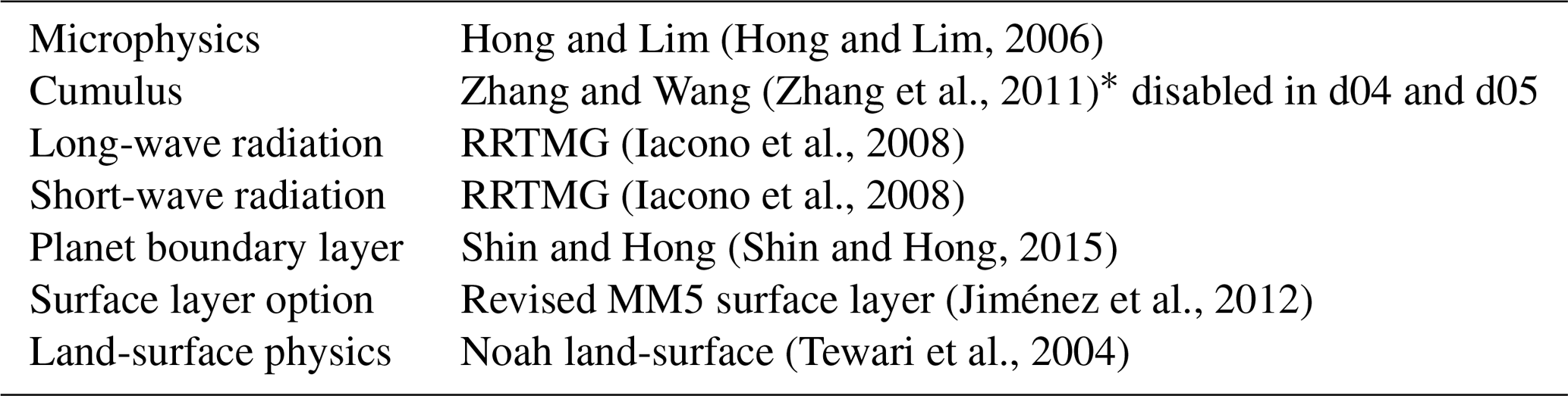
The S–H planetary boundary layer option is more suitable for the high resolution of the innermost domain (444 m) because it helps to mitigate a double counting effect of the small-scale processes in gray-zone resolutions. Apart from this, this scheme provides a turbulent kinetic energy (TKE) diagnostic variable useful for our analyses.
2.2 Global model and real data
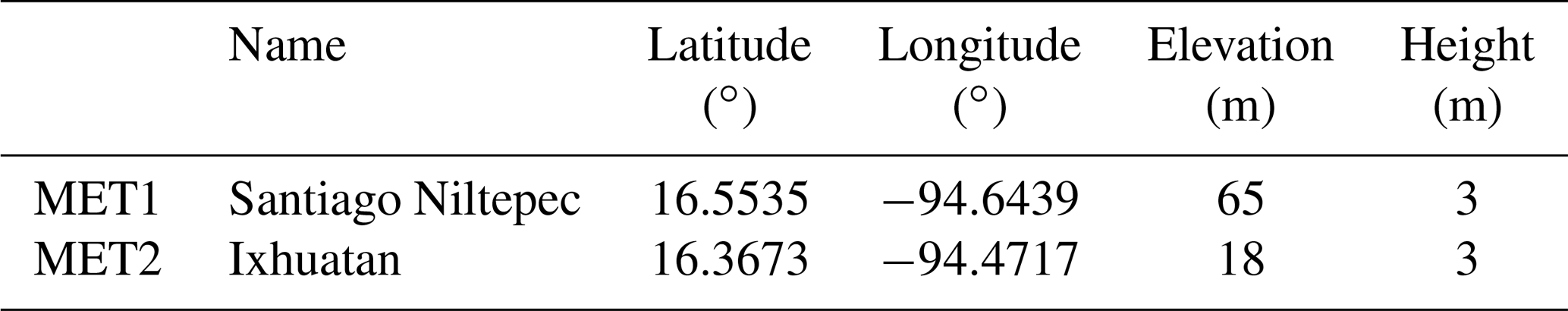
Global Forecast System (GFS) analysis data from the National Centers for Environmental Prediction (NCEP) are used as initial and boundary conditions for the WRF model, with a 3 h update interval. The horizontal resolution of this dataset for all variables is 0.5∘ × 0.5∘ with 32 vertical levels ranging from 1000 to 10 hPa. The observational data used in this work are provided by the Mexican National Laboratory of remote sensors (https://clima.inifap.gob.mx/lnmysr/Estaciones/MapaEstaciones, last access: 10 January 2018), collected every 15 min at two meteorological stations whose locations are presented in Table 2 and marked in Fig. 1b as MET1 and MET2. Wind speed, wind direction and temperature at 3 m height from these points are used for validation.
Model data are extrapolated from their native sigma levels to the height of the meteorological station using Eq. (3), which relates wind speed with friction wind speed, which is also a diagnostic variable in the model.
where U* in the friction velocity, K is the von Kármán constant, z is the height and z0 is the surface roughness (m).
3.1 Synoptic and mesoscale situation
Figure 2 shows the synoptic situation, from GFS analysis data, in North America and Central America 18 h before (Fig. 2a) and at peak intensity of the event (Fig. 2b).
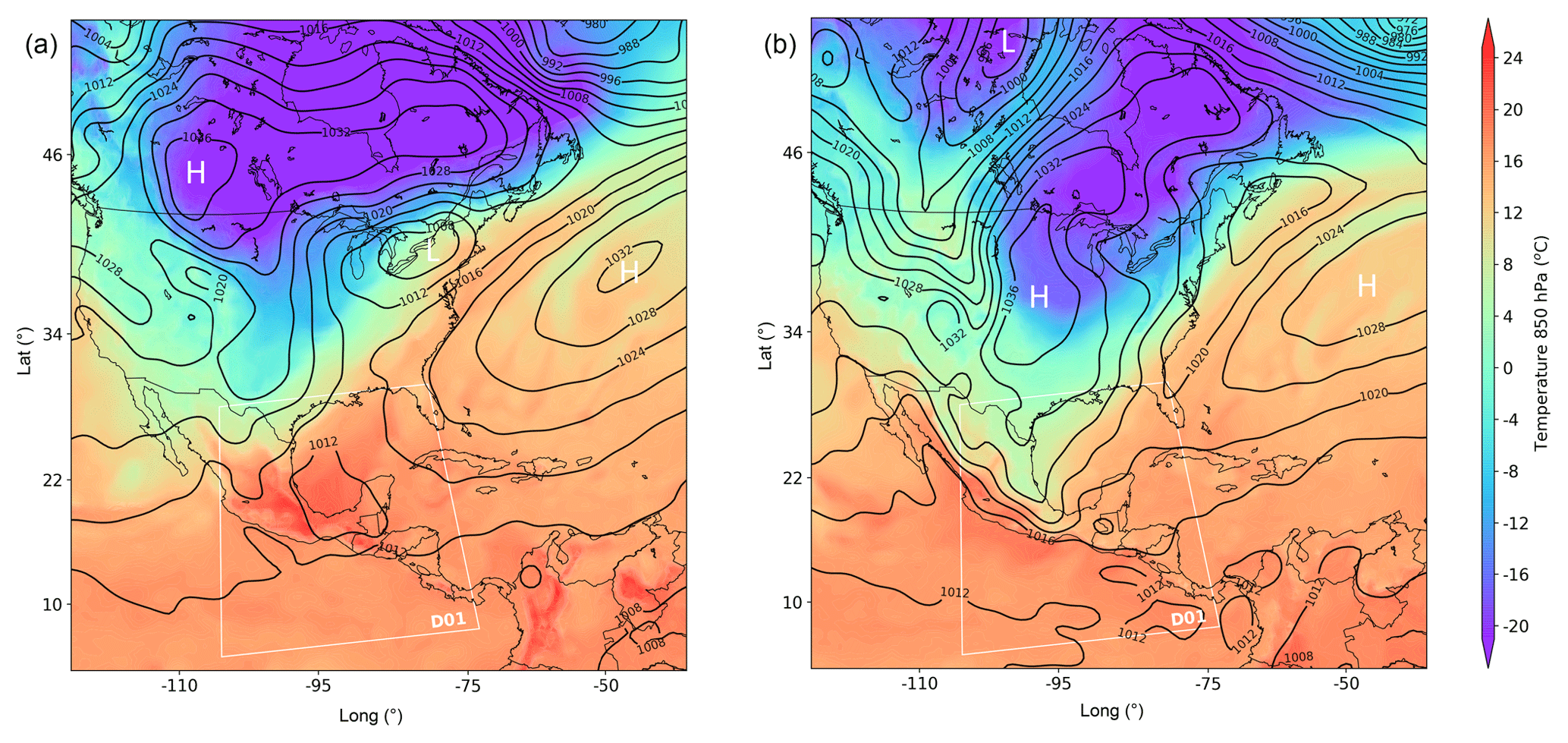
Figure 2(a) 850 hPa temperature (∘C) and sea level pressure (hPa) from GFS 0.5 analysis data at 22 December 2013 18:00 UTC. (b) Same as (a) at 24 December 2013 03:00 UTC. D01 simulation domain is represented with a white square in both cases.
The large-scale setting is typical of Tehuantepecer wind episodes where an Arctic air mass east of the Rockies pushes south across the Great Plains with its leading edge reaching first the Gulf of Mexico (on 22 December, Fig. 2a) and then as far south as the Bay of Campeche (about 1 d later, Fig. 2b), the result of cold air damming east of the Sierra Madre Oriental range in Mexico. The equatorward displacement of the associated high-pressure system on the wake of the cold front creates a strong pressure gradient across the Isthmus of Tehuantepec, ultimately producing the strong mountain gap winds through the low elevation of Chivela Pass. The general situation favoring Tehuantepecer winds persists for about 6 d, more pronounced earlier on.
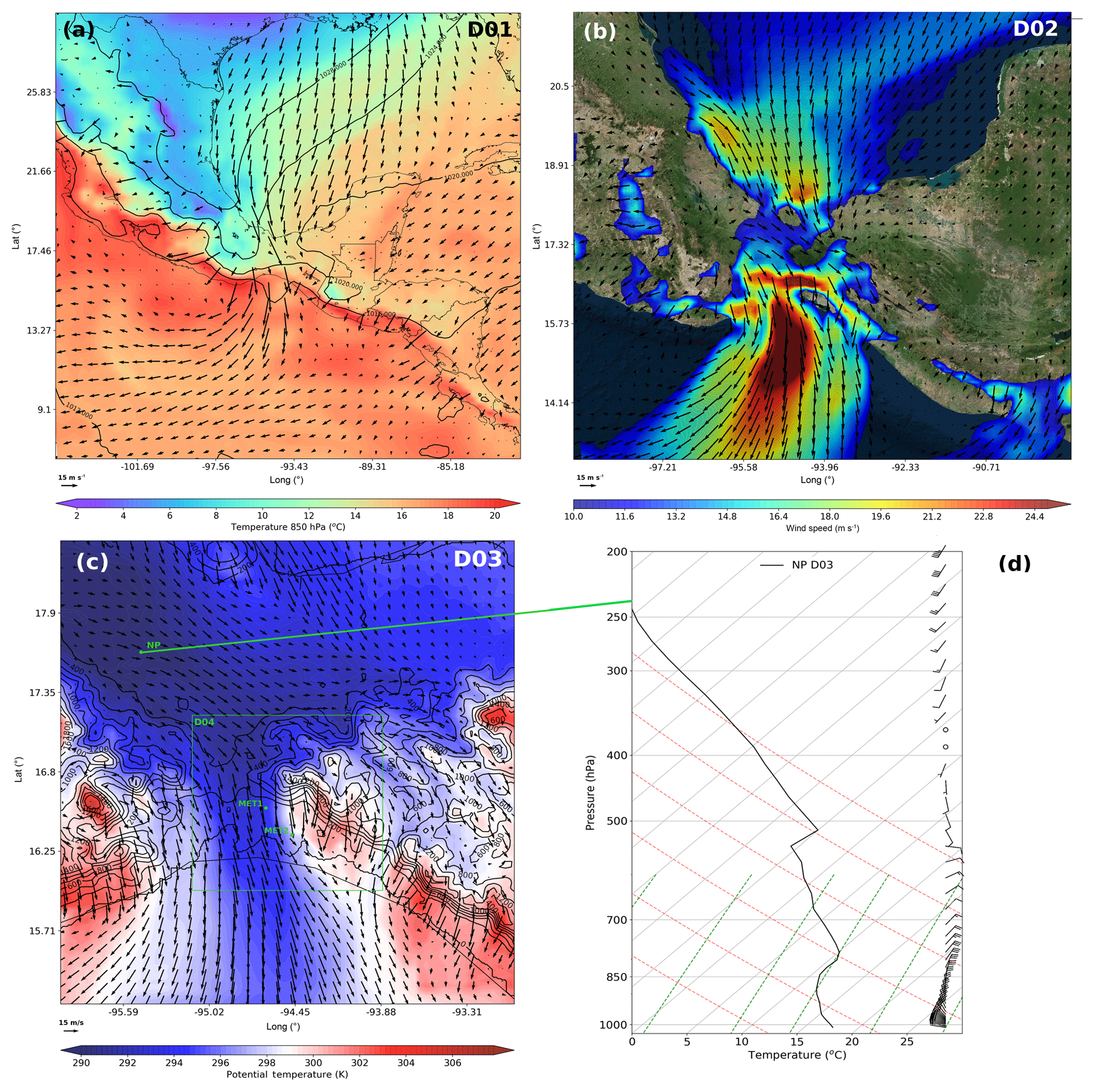
Figure 324 December 2013 03:00 UTC (a) 850 hPa temperature (∘C), sea level pressure (hPa) and wind vectors in the parent grid d01, (b) wind speed (values > 10 m s−1) and wind vectors at σ=3 (about 70 m above ground) in d02, and (c) topography (m, contours) and potential temperature (K, shades) and wind vectors at σ=3 in d03. (d) Skew-T log-P diagram on the Gulf of Mexico side of the isthmus, northeast of Chivela Pass (NP point in c; lat = 17.6463∘, long = −95.6246∘) with wind barb profile at right.
Figure 3 shows the mesoscale conditions of the fully developed extreme wind episode at 03:00 UTC of 24 December 2013 from the WRF simulation. In the coarser grid D01 (36 km spacing, outlined in white in Fig. 2) the cold air damming by the Sierra Madre Oriental is clearly apparent with the northerly cool air mass intrusion extending to the Bay of Campeche, from where it is funneled across the Isthmus of Tehuantepec (Fig. 3a). The higher resolution of the nested grids shows in greater detail the structure of the gap winds. Figure 3b, from the first nested D02 (12 km grid spacing), depicts the wind field (vectors) highlighting in shades the values above 10 m s−1 at about 70 m above the surface (sigma level 3), the approximate height of wind turbine hubs. The strong Tehuano outflow from Chivela Pass reaches velocities of 25 m s−1 as it fans out for more than 100 km into the Pacific Ocean. High wind speeds are not only restricted to the outflow of the mountain gap itself but the simulation results suggest that they also occur in the mountains west and especially east of Chivela Pass. The potential temperature field on the same σ=3 level at the enhanced resolution (4 km) of the next nested grid (D03; Fig. 3c) illustrates how the stable cold air mass to the north surmounts the lower hills neighboring the pass, particularly those to the east where elevation increases more gradually. As shown in the following Sect. 3.2, acceleration on the top of these mountains and to their lee is related to gravity wave activity, which results in the development of strong downslope winds, rotors and HJs. The model sounding at location NP, on the Gulf of Mexico side of the isthmus (Fig. 3d), shows in the temperature profile a stable lower boundary layer capped by a very stable isothermal layer from 850 hPa up to about 2000 to 2500 m, defining the depth of the cold air pool, indeed above the aforementioned mountain tops. A weak inversion associated with the subsidence within the high-pressure system aloft is also clearly apparent just below 500hPa. Above this level, winds are weak and veer from being southeasterly to southwesterly in the upper troposphere. Below 500 hPa, winds back from an easterly to a northeasterly direction at about 800 hPa, and more strongly in lower levels, becoming westerly at the surface, indicating intense cold air advection. There is a pronounced reverse wind shear in the lower troposphere.
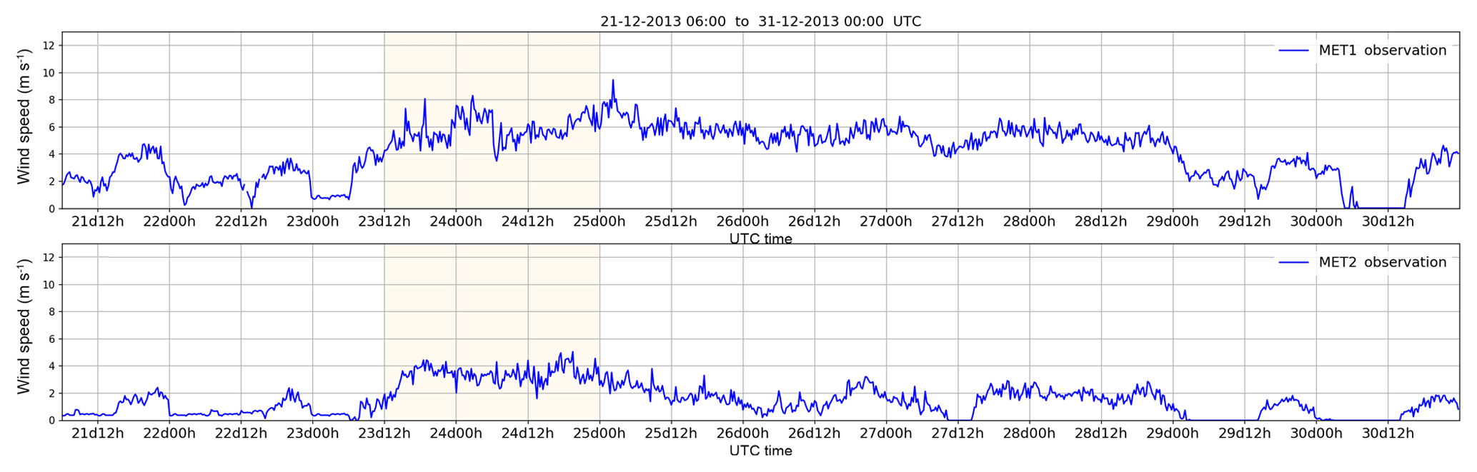
Figure 4Wind speed (m s−1) time series for observation stations MET1 and MET2 (locations marked in Fig. 3). The orange shaded area corresponds to the period simulated.
As mentioned earlier, the only available observations in the area are from stations MET1 and MET2, whose positions are marked in Fig. 3c. They are both located on the Pacific coastal plain, south of the mountains bordering Chivela Pass to the east; MET1 is closer to the relief and further west than MET2. The wind speed time series covering the entire Tehuano episode for both stations is shown in Fig. 4. Wind speeds are low in the previous days and show a daily cycle, likely linked to sea breezes, more clearly evident in station MET2 closer to the coast. The situation changes after about 23 December 06:00 UTC when, picking up intensity, wind speeds become more constant throughout the day, the signature of a Tehuano wind occurrence. At about 00:00 UTC on 29 December, the episode decays and winds go back to local breeze regimes. The extent of the simulated period covers the first 36 h of the event (shaded in Fig. 4), corresponding with its highest intensity in both locations. These observations away from Chivela Pass show evidence, as the simulations suggest, that the neighboring mountains may also induce strong winds, even though they certainly do not reach out as far as the mountain gap outflow does.
3.2 Upstream–downstream structure
In this section, we focus on the fine-scale structure of the flow acceleration across the isthmus, and more precisely on that occurring on the westernmost section of the Sierra Madre de Chiapas bordering Chivela Pass, apart from the well-known strong gap wind jet. This is the area covered by the d04 domain of 1.3 km resolution (highlighted in green in Fig. 3c), encompassing with 137 km from north to south the wind flow path before and after crossing the mountains. Figure 5 depicts, from d04, latitudinal cross sections (red lines in Fig. 1b) facing east (south to the left, north to the right) of different variables at the longitude of the two validation points MET1 (Fig. 5a–f) and MET2 (Fig. 5g–l).
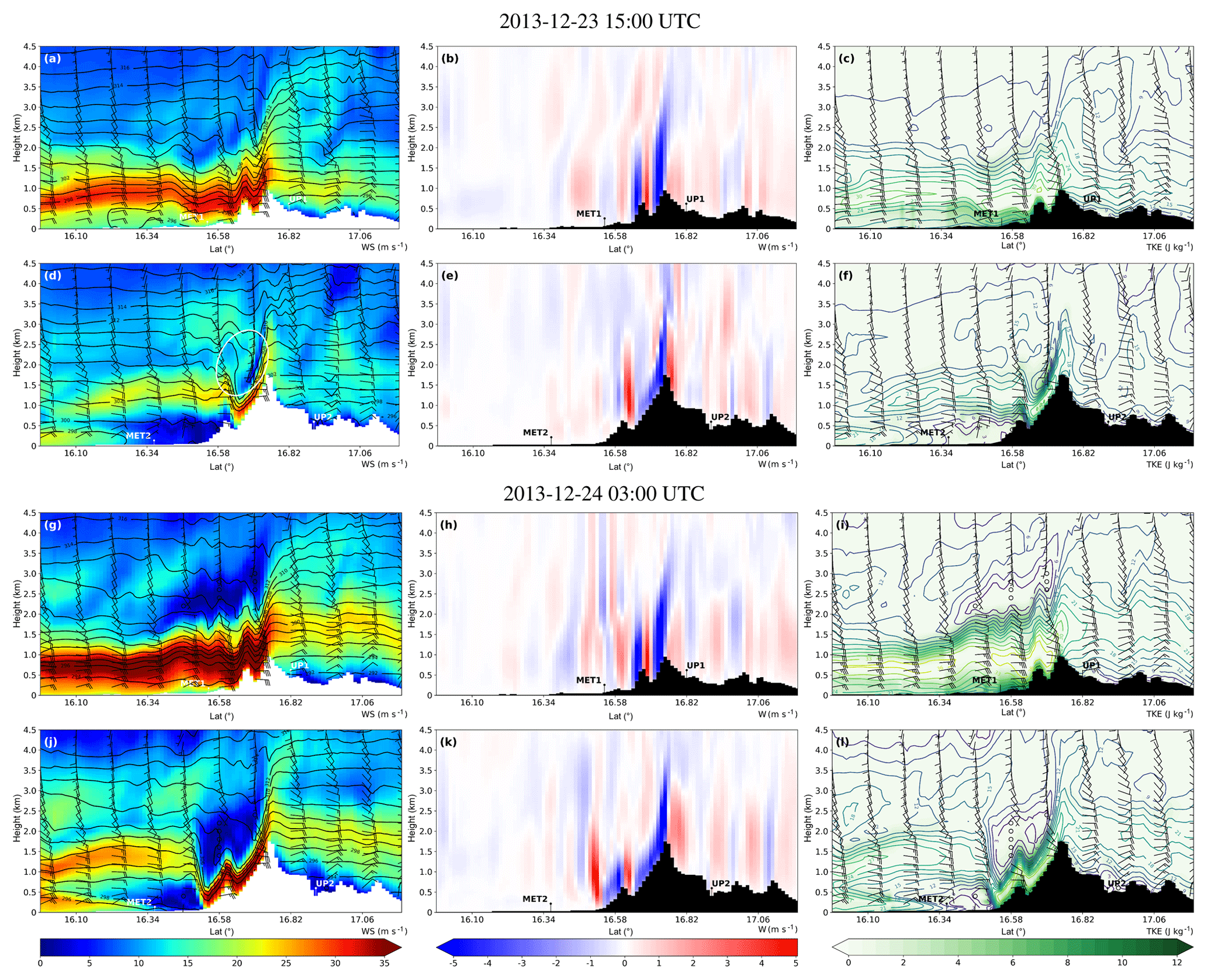
Figure 5d04 vertical cross sections (a, d, g, j) of potential temperature (K, contours), wind speed (m s−1 shades), and wind barbs referenced to the orientation of the cross section plane, (b, e, h, k) vertical wind component W (m s−1) and (c, f, i, l) wind speed (m s−1) isolines and turbulent kinetic energy (TKE, J kg−1, shades). Panels (a–c) for MET1 and (d–f) for MET2 correspond to the initial stages of the episode on 23 December 2013 15:00 UTC. Panels (f, h, i) at MET1 and (j, k, l) at MET2 are for the fully developed events on 24 December 2013 03:00 UTC. UP1 and UP2 are the locations where the Froude number upstream the mountain is calculated.
The tight isentropes on the windward side of the mountains (to the right in Fig. 5a, d, g and j), indicate a quite similar stable stratification in the whole lower tropospheric column in both cases, stronger in the layers below about 2.5 km and weaker above. The temperature profile in Fig. 3d show evidences that the 2500 m height level corresponds to the depth of the cold air. Winds are northerly in these lower layers to the north of the mountains with somewhat higher speeds above 20 m s−1 upstream from MET1 than further east, north of MET2. In both cases, winds above the cool pool are much weaker, and back to an easterly component at about 4000 m and above. The latter height is therefore a critical level since the cross-mountain flow component becomes null; thus, triggered gravity waves will break and dissipate when they approach it. Markowski and Richardson (2010) outline seven conditions conducive to DSWS, albeit not all of them absolutely necessary. These conditions are (1) an asymmetric mountain with steeper lee than windward side (Fig. 5), (2) crossed by strong winds (>15 m s−1) (Fig. 5), with (3) winds mostly normal to the barrier (Figs. 3 and 5), (4) a stable layer above the top and less stable above that (Figs. 3d and 6c), and with (5) cold air advection and large-scale subsidence to maintain the stability (Figs. 3d and 6c). Apart from this, (6) reverse wind shear above (Figs. 3d and 6c) and (7) no cool pool in the lee (Figs. 3a and 6b) are also desirable. These conditions are all perfectly met for both locations analyzed, as discussed previously, and indeed intense DSWSs occur in both cases.
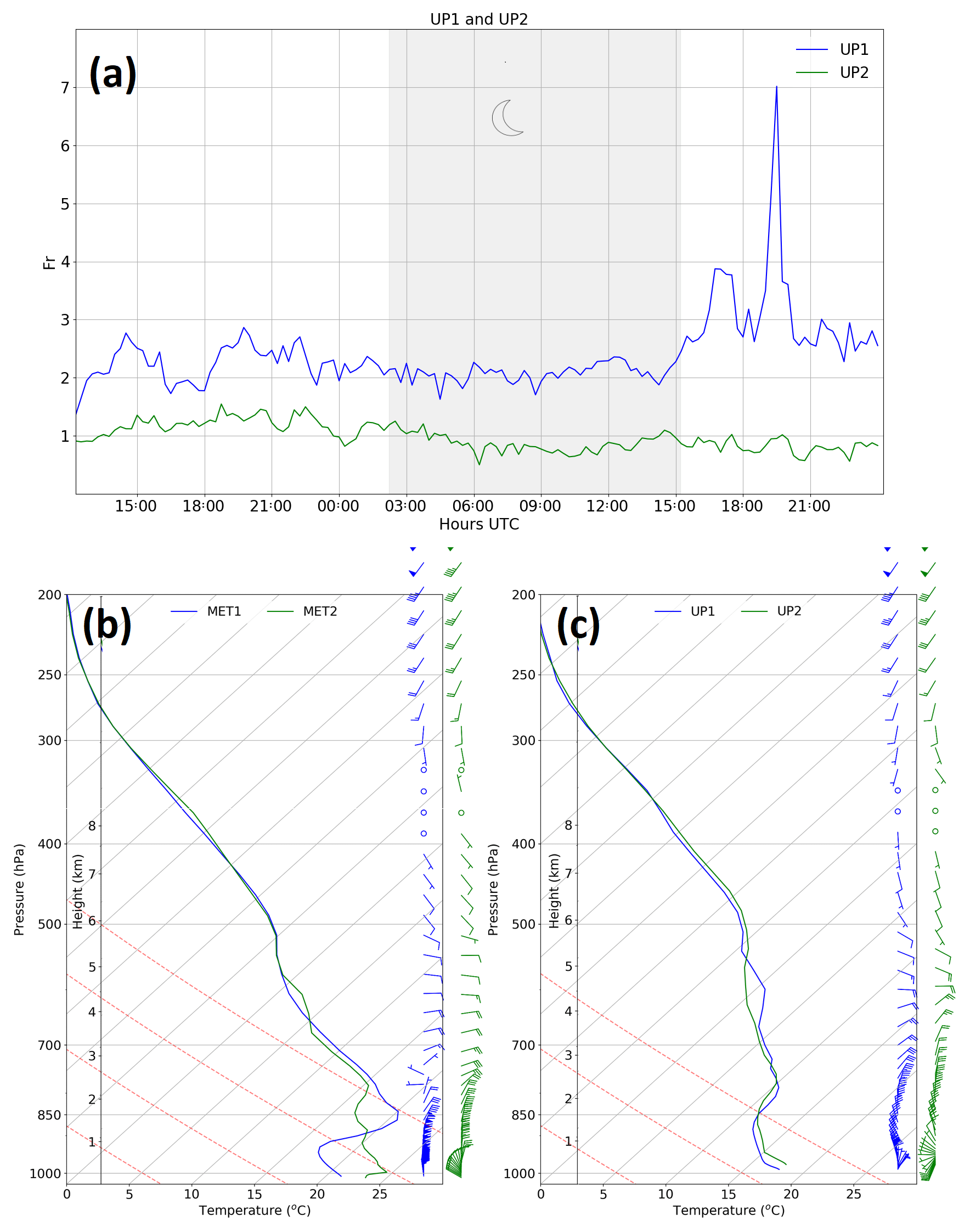
Figure 6(a) Froude number upstream of the mountain, north of MET1 (UP1) and of MET2 (UP2). The gray zone represents nighttime. (b) Skew-T log-P diagram at MET1 and MET2 and (c) at their corresponding upstream points UP1 and UP2. Wind barb profile for each pair of points at right.
The stably stratified cross-barrier flow displays wave activity from early on, and wave breaking, as the vertical isentropes suggest (Fig. 5a and d), enhances turbulent mixing (Fig. 5c and f), and yields a region of weak stability and reverse flow immediately downwind from the mountain crests (Fig. 5g and j). In both cases, isentropes on the windward side sink sharply under these layers of low stability on the lee side, much more pronouncedly for the tallest mountain (Fig. 5j). Encompassing the well-mixed region to the lee, a split streamline develops (Smith, 1985b) and below its lower branch there is flow thinning and a significant increase in wind speed. However, the particular features existent on the lee side differ, depending of the height of the topographic obstacle. The strong accelerated flow confined by layers of strong wind shear and turbulence extends for many kilometers downwind from the lowest mountain (Fig. 5i), while ending with a HJ and rotors at the foot when the barrier is higher (Fig. 5j). The formation of either of these lee wave events is related to the Froude number upstream (Smith, 1989). We note that only the turbulence produced by the existent wind shear in the column is well captured in the simulation (Fig. 5i and l). The subgrid-scale turbulence associated with gravity waves due to rotors and nonlocal turbulent advection or with instability resulting from wave overturning is not represented and accounted for since a much higher horizontal and vertical resolution on the order of tens of meters would be needed in order to explicitly resolve these features (Vosper et al., 2018).
Figure 6a plots the Froude number (Eq. 2) calculated using the average of the variables at sigma levels from the ground to the mountain top at upstream points UP1 (MET1 case) and 2 (MET2 case). For the lowest mountain, Fr≈2 during nighttime and even higher at some other times during the day, indicating supercritical conditions. The Brunt–Väisälä frequency around mountain top is between 0.020 and 0.025 s−1. The generated mountain waves have relatively short wavelength and small amplitude and a modest HJ that propagates downstream can be seen at the initial stages of the episode at 15:00 UTC 23 December (Fig. 5a). Some 12 h later, during nighttime, the aforementioned strong jet extending for tens of kilometers downwind is fully formed with values above 35 m s−1 at about 750 m above ground and strong turbulence at the surface and in the layers above the jet, where stability is much reduced. The temperature profile upwind (at 03:00 UTC 24 December and location UP1 in Fig. 5) shows in the temperature profile a stable lower boundary layer capped by a very stable isothermal layer from 850 hPa up to about 800 hPa, or 2500 m, defining the depth of the cold air pool. At the observation location MET1, downwind from the mountain, the lowest layers up to about 900 m are well mixed (slightly lower, up to 750 m further downstream), a result of the intense surface turbulence. Above the latter height and up to about 1500 m elevation, a strongly stable layer exists corresponding with the aforementioned packing of the isentropes (and streamlines). This is where the highest wind speeds are found. Stability is sharply reduced aloft, in the region encompassed by the dividing streamline, and winds are rather weak and have an easterly component for the most part, parallel to the mountains.
For the higher mountain north of MET2, Fr≈1 consistently in the period, indicating a critical flow regime prone to the formation of HJs (Vosper2006, 5B). The Brunt–Väisälä frequency around mountain top is between 0.012 and 0.015 s−1 and the generated waves have higher amplitudes than in the MET1 case. Wave overturning and breaking is also much more pronounced (Fig. 5d, highlighted in white) and the well-mixed region forming to the lee of the crest is deeper. Isentropes and streamlines that sink underneath this region are packed in a very shallow layer on the lee slope of the mountain, generating an intense DSWS with speeds above 35 m s−1 at the surface. These strong winds end abruptly at the foot of the hill, where the flow transitions to subcritical conditions and a marked stationary HJ forms, with vertical wind speeds of 6 m s−1. A rotor extending from the jump to the location of observation station MET2 is also evident in Fig. 5l. The temperature profile upstream is very similar to that of the MET1 case, but downwind from the mountain at location MET2 lacks the strongly stratified layer present in the case of the lower mountain. We note that the soundings in Fig. 6 show complex temperature profiles with discontinuous stratification in the planetary boundary layer, which underscores the importance of using high vertical resolution in simulations for these kinds of studies.
Results from the innermost nested grid d05 with the finest resolution (Fig. 7) suggest that trapped lee waves develop in the MET1 case within the high-stability layer where the strongest winds are found, just below the low-stability region and the critical level aloft that prevent their vertical propagation. This wavelike pattern is a common feature in DSWS periods (Pokharel et al., 2017b; Hertenstein and Kuettner, 2005) and fully formed 12 h later (Fig. 7c), extends for more than 100 km downstream aligned with the general orientation in the northwest–southeast direction of the Sierra in the region. Waves are absent further east in the MET2 cross section, where the topographic barrier is higher and a stationary HJ forms instead, as discussed above.
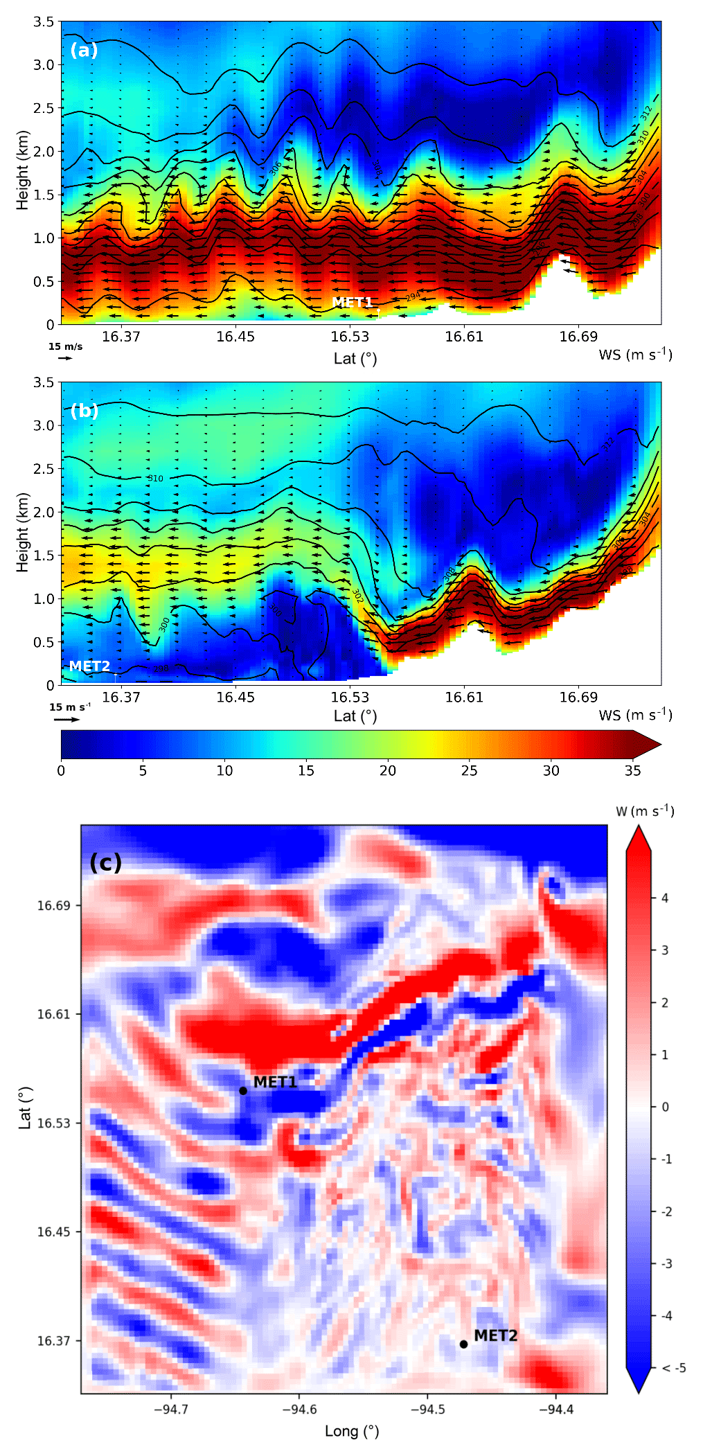
Figure 7As in Fig. 5g and j but for d05 vertical cross sections of potential temperature (K, contours), wind speed (m s−1 shades) and wind barbs referenced to the orientation of the cross section plane at 24 December 2013 03:00 UTC for (a) MET1 and (b) MET2. (c) Vertical wind speed (m s−1) in d05 at sigma level 17 (about 1400 m above ground) when the trapped lee wave pattern in the region is fully formed at 15:30 UTC 24 December 2013.
Our results suggest that during Tehuano wind events, the Pacific side of the Isthmus of Tehuantepec east of Chivela Pass is very prone to host extreme wind phenomena. The formation of DSWSs in the area increases the impacts of the already strong mountain gap winds.
3.3 Validation
Finally, we contrast our simulation results with the very few data available for validation at meteorological stations MET1 and MET2. The two plots in Fig. 8 compare the simulated wind speed (in d04 and d05) with observations from both stations.
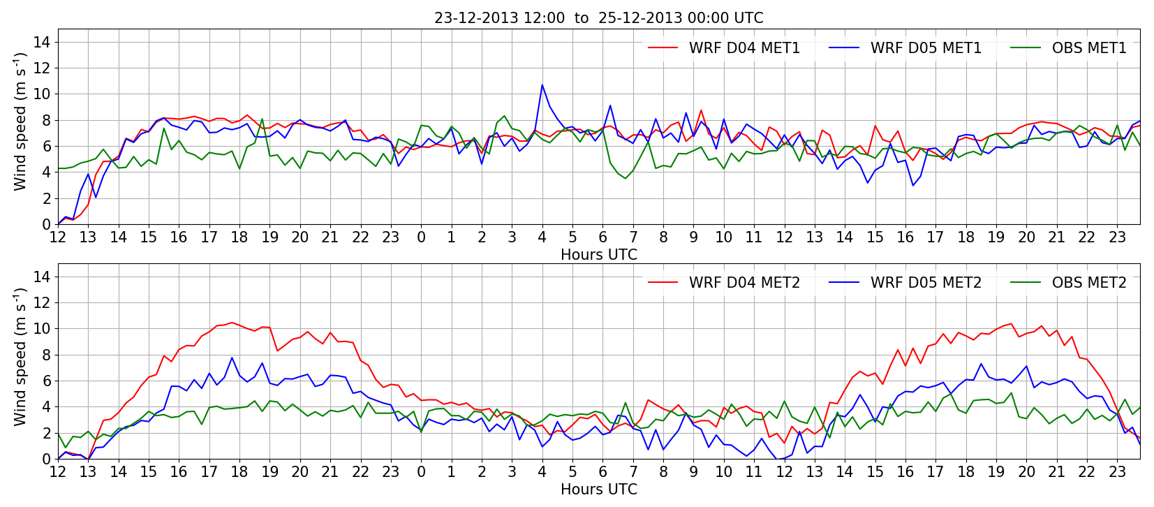
Figure 8(a) Wind speed comparison among observations at MET1 (green), and model output from d04 (red), and d05 (blue). (b) Same for station location MET2.
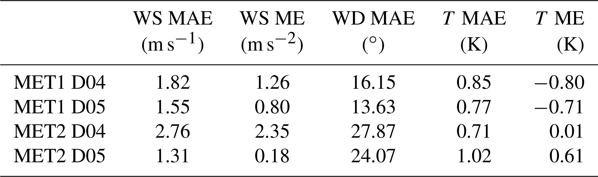
Wind speed results from d04 and d05 at location MET1 are quite similar, and fare well with respect to observations (Fig. 8a), slightly better in the d05 case with a mean absolute error (MAE) of 1.55 m s−1 (Table 3). The similarity in the low mean error between both simulations and their high correlation throughout the period are due to the nature of the event in that area, an intense and mostly steady jet that the d04 domain resolution (1.3 km) is already capable of resolving accurately. However, results in MET2, downwind from the strong HJ, present more differences between d04 and d05 (Fig. 8b) and there is a significant improvement in d05 with respect to its parent domain d04. Wind speeds in d04 are overestimated (mean error ME = 2.76 m s−1) and present a daily cycle that is absent or very subtle in the observations. The complexity and fast variability in HJ formation in this area are better resolved in the higher-resolution grid, which perhaps reproduces more accurately the stagnant flow and rotor formations downstream from the HJ. With regard to wind direction, errors are small for MET1 and significantly higher for MET2 due to the same reasons. As in the case of wind speeds, wind direction results from the finer grid d05 are also better than in d04. Temperature errors are equal or below 1 K in both locations and domains, hence the surface thermal evolution is well captured.
Table 3Wind speed (WS), wind direction (WD), and temperature (T) mean errors (ME) and mean absolute errors (MAE) at MET1 and MET2 locations during the simulated period and for the two higher-resolution domains (d04 and d05).
Lee waves can promote orographic cloud formation at different scales, depending on the amplitude of the wave and elevation (Armi and Mayr, 2011; Szmyd, 2016). Model results in d05 suggest that lenticular clouds form at the crests of the trapped lee waves depicted in Fig. 7. Figure 9a shows a 3-D representation of the modeled cloud water mixing ratio at 24 December 2013 15:30 UTC in d05. Cross sections of wind speed at the surface observation locations MET1 and MET2 as in Figs. 5 and 7 are also included for reference. A 2-D view of the same cloud mixing ratio variable and wind vectors at sigma level 17 (about 1400 m above ground), revealing existing clouds, are depicted overlaying a satellite image of the area. An actual satellite image from Geostationary Operational Environmental Satellite – R Series (GOES-R) (http://www.goes-r.gov/education/docs/fs_imagery.pdf, last access: 15 September 2018) around the same time is shown for comparison, indicating that remarkably similar mountain wave cloud formations were indeed observed in the area. The actual existence of these lenticular clouds with the same location and pattern as in the simulation further validates the model results.
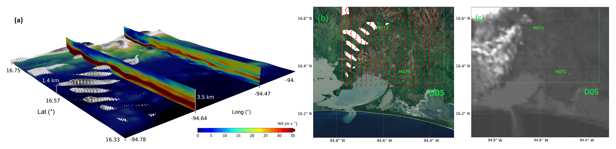
Figure 9(a) Cloud water mixing ratio 3-D representation in d05 at 24 December 2013 15:30 UTC. The two cross sections show the N–S wind profile at the longitudes of the meteorological stations MET1 and MET2. (b) Satellite image of the terrain in d05 and cloud water mixing ratio (white shades) and wind vectors at about 1.4 km above ground. (c) GOES-R satellite image on 24 December 2013 20:30 UTC, revealing very similar lenticular cloud formations at the same locations.
In the present work, we studied lee wave phenomena occurring during Tehuano events on the Pacific side of the Isthmus of Tehuantepec using WRF high-resolution simulations. Orographic forcings at different scales result in the well-known gap wind jet off Chivela Pass, but also in downslope windstorms and hydraulic jumps in the neighboring mountains. We analyzed these phenomena in an episode in December 2013 having the typical genesis of Tehuantepecer wind events. An Arctic air mass in North America pushed as far south as the Bay of Campeche due to cold air damming east of the Rockies continuing to the east of the Sierra Madre Oriental range in Mexico. The displacement of the associated high-pressure system on the wake of the cold front created large pressure differences across the Isthmus of Tehuantepec, ultimately producing the strong mountain gap winds through the low elevation of Chivela Pass. The model simulates these intense winds, blowing with speeds at the surface of more than 25 m s−1 that extend for many kilometers from the mountain gap, fanning out well into the Gulf of Tehuantepec, as it is commonly observed in Tehuano events (Steenburgh et al., 1998).
The depth of the cold surge on the coastal plains of the Gulf of Mexico side of the isthmus is about 2500 m; therefore, thick enough to surmount the lower elevations to the west and especially to the east of Chivela Pass. The flow over these mountains results in intense DSWSs to their lee with the generation of intense turbulence, HJs and rotors, depending on the particular height of the topography. We focus on two locations of different barrier elevation from where there are surface observations downwind: one of 963 m closer to Chivela Pass and another further east, with height increasing to 1736 m.
The thermodynamic characteristics of the air masses are rather uniform upwind of both mountains, with strong stability within the cool pool and weaker above, and intense northerly winds that back and weaken aloft to a more easterly component parallel to the barrier. The critical level where the cross-mountain wind component becomes zero, inhibiting wave propagation, is about 4000 m. Mountain waves are generated in both cases, with smaller amplitudes for the lower mountain, where the Brunt–Väisälä frequency at crest height is between 0.020 and 0.025 s−1, than for the higher mountain, where the Brunt–Väisälä frequency is about half. Wave breaking produces mixing and generates a region of low stability to the lee of the mountains, which is deeper where the waves have higher amplitude. The Froude number is around 2.5 at crest height in the lower barrier and the flow presents a supercritical behavior. The region of low stability to the lee of the mountain lies above about 1500 m and leads to a packing of the isentropes and streamlines underneath, resulting in strong stability and flow acceleration. An intense jet develops with wind speeds of 35 m s−1 at about 750 m above ground extending for tens of kilometers downwind from the mountains. Wind speeds are reduced closer to the surface due to intense turbulence. Trapped lee waves form at about 1500 m, just below the well-mixed layer aloft that prevents their vertical propagation. The Froude number decreases to about 1 further east as elevation rises and the flow presents a critical regime. Isentropes on the windward side of the mountain sink much more pronouncedly under the wider mixed layer generated by wave breaking to the lee, and are tightly packed in a shallow layer above the surface. This generates an intense wind storm on the lee slope of the mountain with surface wind speeds up to 35 m s−1. The accelerated flow down the mountain ends abruptly at its foot, where the flow turns to subcritical state and a marked stationary HJ forms, with vertical velocities of 6 m s−1. A rotor circulation develops further downstream from the jump.
Only limited observations are available to validate our model results. Errors in surface wind speeds, directions and temperature are small at the only two stations available on the Pacific coastal plain downwind from the mountains. In addition, lenticular clouds, similar in location and pattern to those produced by the model, are apparent in satellite imagery of the day of the event, providing valuable indication that the mountain lee wave phenomena simulated indeed correspond to a real scenario.
Our model results suggest that when the cold air mass intruding from the north on the Gulf of Mexico side of the isthmus is thick enough to surmount the mountains, extreme wind events develop in the area during Tehuano events beyond the gap wind jet. These include DSWSs and HJs, which are intense and highly turbulent flows that can have a substantial impact on the existent wind farm industry in the region.
Observational data from meteorological stations can be requested from the Mexican national laboratory of remote sensors at https://clima.inifap.gob.mx/lnmysr/Estaciones/MapaEstaciones (last access: 10 January 2018). Geostationary Operational Environmental Satellite – R Series (GOES-R) data can be downloaded for free at https://www.ngdc.noaa.gov/stp/satellite/goes-r.html (last access: 10 January 2018).
The supplement related to this article is available online at: https://doi.org/10.5194/esd-10-485-2019-supplement.
MAP, IST and GMM designed the research. MAP and COC performed the simulations with the WRF model in CESGA computing facilities. MAP, COC and GMM analyzed the data. MAP and GMM drafted the paper. MAP designed all the figures. All authors contributed to the interpretation of the data and revision of the paper.
The authors declare that they have no conflict of interest.
We would like to thank the Mexican National Laboratory of remote sensors (INAFAP) (http://clima.inifap.gob.mx/lnmysr/, last access: 20 January 2018) for the valuable real data provided, necessary to validate all of the study. The model forecast simulations and development of the data analysis were performed at the Centro de Supercomputacion de Galicia (CESGA) (http://www.cesga.es/, last access: 10 January 2019). Their computer facilities and support have been indispensable to carry out this project. Finally, we would like to acknowledge the Nonlinear Physics Group of Universidade de Santiago de Compostela (http://www.usc.es/en/investigacion/grupos/gfnl, last access: 10 January 2019), which is where this whole project has been developed.
This paper was edited by Zhenghui Xie and reviewed by three anonymous referees.
Ágústsson, H. and Ólafsson, H.: Simulations of Observed Lee Waves and Rotor Turbulence, Mon. Weather Rev., 142, 832–849, https://doi.org/10.1175/MWR-D-13-00212.1, 2014. a
Armi, L. and Mayr, G. J.: The descending stratified flow and internal hydraulic jump in the lee of the Sierras, J. Appl. Meteorol. Clim., 50, 1955–2011, https://doi.org/10.1175/JAMC-D-10-05005.1, 2011. a
Bacmeister, J. and Pierrehumbert, R.: On high-drag states of nonlinear stratified flow over an obstacle, J. Atmos. Sci., 45, 63–80, 1988. a
Baines, P. G.: Upstream blocking and airflow over mountains, Annu. Rev. Fluid Mech., 19, 75–95, 1987. a
Baxter, R., Hastings, N., Law, A., and Glass, E. J.: Prospectiva de Energías Renovables 2017–2031, Tech. Rep. 5, Subsecretaría de Planeación y Transición Energética, Secretaria de Energia (SENER), Mexican Goberment, Mexico, available at: https://www.gob.mx/cms/uploads/attachment/file/284342/Prospectiva_de_Energ_as_Renovables_2017.pdf (last access: 20 September 2018), 2017. a
Bontemps, S., Defourny, P., Radoux, J., Van Bogaert, E., Lamarche, C., Achard, F., Mayaux, P., Boettcher, M., Brockmann, C., Kirches, G., Zülkhe, M., Kalogirou, V., Seifert, F., and Arino, O.: Consistent global land cover maps for climate modelling communities: current achievements of the ESA' and cover CCI, in: Proc. “ESA Living Planet Symposium 2013”, 9–13 September 2013, Edinburgh, UK, 9–13, 2013. a
Brennan, M. J., Cobb, H. D., and Knabb, R. D.: Observations of Gulf of Tehuantepec Gap Wind Events from QuikSCAT: An Updated Event Climatology and Operational Model Evaluation, Weather Forecast., 25, 646–658, https://doi.org/10.1175/2009WAF2222324.1, 2010. a, b
Cao, Y. and Fovell, R. G.: Downslope Windstorms of San Diego County. Part I: A Case Study, Mon. Weather Rev., 144, 529–552, https://doi.org/10.1175/MWR-D-15-0147.1, 2016. a
Clark, T. and Peltier, W.: On the evolution and stability of finite-amplitude mountain waves, J. Atmos. Sci., 34, 1715–1730, 1977. a
Coldwell, P. J., Ricardo, A., Quiroga, F., and Reyes, F. Z.: Reporte de Avance de Energias Limpias 2017, Tech. rep., Subsecretaría de Planeación y Transición Energética, Secretaria de Energia (SENER), Mexican Goberment, Mexico, avaliable at: https://www.gob.mx/cms/uploads/attachment/file/340121/Informe_Renovables_2017_cierre.pdf (last access: 20 September 2018), 2017. a
Durran, D. R.: Another look at downslope windstorms. Part I: The development of analogs to supercritical flow in an infinitely deep, continuously stratified fluid, J. Atmos. Sci., 43, 2527–2543, 1986a. a
Durran, D. R.: Another look at downslope windstorms. Part I: The development of analogs to supercritical flow in an infinitely deep, continuously stratified fluid, J. Atmos. Sci., 43, 2527–2543, 1986b. a
Durran, D. R.: Mountain waves and downslope winds, in: Atmospheric processes over complex terrain, American Meteorological Society, Boston, MA, 59–81, 1990. a
Durran, D. R. and Klemp, J. B.: Another look at downslope winds. Part II: Nonlinear amplification beneath wave-overturning layers, J. Atmos. Sci., 44, 3402–3412, 1987. a
Grubišić, V., Serafin, S., Strauss, L., Haimov, S. J., French, J. R., and Oolman, L. D.: Wave-induced boundary-layer separation in the lee of the Medicine Bow Mountains. Part II: Numerical modeling, J. Atmos. Sci., 72, 4865–4884, https://doi.org/10.1175/JAS-D-14-0376.1, 2015. a
Hernández, J.: Motorista pierde la vida en accidente sobre carretera 190, El Imparcial de Istmo, available at: http://imparcialoaxaca.mx/policiaca/245626/motociclista-pierde-la-vida-en-accidente-sobre-carretera-190/, last access: 15 December 2018. a
Hertenstein, R. F. and Kuettner, J. P.: Rotor types associated with steep lee topography: Influence of the wind profile, Tellus A, 57, 117–135, https://doi.org/10.1111/j.1600-0870.2005.00099.x, 2005. a
Hong, S. and Lim, J.: The WRF single-moment 6-class microphysics scheme (WSM6), available at: http://www.mmm.ucar.edu/wrf/users/docs/WSM6-hong_and_lim_JKMS.pdf\%5Cnhttp://search.koreanstudies.net/journal/thesis_name.asp?tname=kiss2002&key=2525908 (last access: 1 June 2018), 2006. a
Hong, X., Peng, M., Wang, S., and Wang, Q.: Simulating and understanding the gap outflow and oceanic response over the Gulf of Tehuantepec during GOTEX, Dynam. Atmos. Oceans, 82, 1–19, https://doi.org/10.1016/j.dynatmoce.2018.01.003, 2018. a
Iacono, M. J., Delamere, J. S., Mlawer, E. J., Shephard, M. W., Clough, S. A., and Collins, W. D.: Radiative forcing by long-lived greenhouse gases: Calculations with the AER radiative transfer models, J. Geophys. Res.-Atmos., 113, 2–9, https://doi.org/10.1029/2008JD009944, 2008. a, b
Francisco Ibáñez, S.: El potencial eólico mexicano. Oportunidades y retos en el nuevo sector eléctrico, Asociación Mexicana de Energía Eólica (AMDEE), available at: https://www.amdee.org/Publicaciones/AMDEE-PwC-El-potencial-eolico-mexicano.pdf, last access: 15 September 2018. a
Jaramillo, O. A. and Borja, M. A.: Wind speed analysis in La Ventosa, Mexico: A bimodal probability distribution case, Renewable Energy, 29, 1613–1630, https://doi.org/10.1016/j.renene.2004.02.001, 2004. a
Jiménez, P. A., Dudhia, J., González-Rouco, J. F., Navarro, J., Montávez, J. P., and García-Bustamante, E.: A Revised Scheme for the WRF Surface Layer Formulation, Mon. Weather Rev., 140, 898–918, https://doi.org/10.1175/MWR-D-11-00056.1, 2012. a
Jung-Hoon, K. and Chung, I.-U.: Study on Mechanisms and Orographic Effect for the Springtime Downslope Windstorm over the Yeongdong Region Jung-Hoon, Atmosphere, 16, 67–83, 2006. a
Klemp, J. and Durran, D.: Numerical modelling of Bora windsNumerische Modellierung der Bora, Meteorol. Atmos. Phys., 36, 215–227, 1987. a
Long, R. R.: Some aspects of the flow of stratified fluids: I. A theoretical investigation, Tellus, 5, 42–58, 1953. a
Markowski, P. and Richardson, Y.: Mesoscale meteorology in midlatitudes, in: Vol. 2, John Wiley & Sons, https://doi.org/10.1002/qj.817, 2010. a
McCreary, J. P., Lee, H. S., and Enfield, D. B.: The response of the coastal ocean to strong offshore winds: With application to circulations in the Gulfs of Tehuantepec and Papagayo, J. Mar. Res., 47, 81–109, https://doi.org/10.1357/002224089785076343, 1989. a
Pokharel, A. K., Kaplan, M. L., and Fiedler, S.: Subtropical Dust Storms and Downslope Wind Events, J. Geophys. Res.-Atmos., 122, 10191–10205, https://doi.org/10.1002/2017JD026942, 2017a. a
Pokharel, B., Geerts, B., Chu, X., and Bergmaier, P.: Profiling radar observations and numerical simulations of a downslopewind storm and rotor on the lee of the Medicine Bow mountains in Wyoming, Atmosphere, 8, 39, https://doi.org/10.3390/atmos8020039, 2017b. a, b
Powers, J. G., Klemp, J. B., Skamarock, W. C., Davis, C. A., Dudhia, J., Gill, D. O., Coen, J. L., Gochis, D. J., Ahmadov, R., Peckham, S. E., Grell, G. A., Michalakes, J., Trahan, S., Benjamin, S. G., Alexander, C. R., Dimego, G. J., Wang, W., Schwartz, C. S., Romine, G. S., Liu, Z., Snyder, C., Chen, F., Barlage, M. J., Yu, W., and Duda, M. G.: The weather research and forecasting model: Overview, system efforts, and future directions, B. Am. Meteorol. Soc., 98, 1717–1737, https://doi.org/10.1175/BAMS-D-15-00308.1, 2017. a
Priestley, M. D., Pinto, J. G., Dacre, H. F., and Shaffrey, L. C.: The role of cyclone clustering during the stormy winter of 2013/2014, Weather, 72, 187–192, https://doi.org/10.1002/wea.3025, 2017. a
Prtenjak, M. T. and Belusic, D.: Formation of reversed lee flow over the north-eastern Adriatic during bora, Geofizika, 26, 145–155, https://doi.org/10.1016/j.memsci.2006.03.045, 2009. a
Rodríguez, Ó.: Viento provoca voladura de camión en Oaxaca, Milenio, available at: http://www.milenio.com/estados/viento-provoca-volcadura-de-camion-en-oaxaca, last access: 15 December 2018. a
Romero-Centeno, R., Zavala-Hidalgo, J., Gallegos, A., and O'Brien, J. J.: Isthmus of tehuantepec wind climatology and ENSO signal, J. Climate, 16, 2628–2639, https://doi.org/10.1175/1520-0442(2003)016<2628:IOTWCA>2.0.CO;2, 2003. a
Santiago, A.: Atendió Protección Civil más de 20 reportes en el Istmo por fuertes vientos, El Imparcial de Istmo, available at: http://imparcialoaxaca.mx/istmo/245475/atendio-proteccion-civil-mas-de-20-reportes-en-el-istmo-por, last access: 15 December 2018. a
Sheridan, P. F. and Vosper, S. B.: A flow regime diagram for forecasting lee waves, rotors and downslope winds, Meteorol. Appl., 13, 179–195, https://doi.org/10.1017/S1350482706002088, 2006. a, b
Shin, H. H. and Hong, S.-Y.: Representation of the Subgrid-Scale Turbulent Transport in Convective Boundary Layers at Gray-Zone Resolutions, Mon. Weather Rev., 143, 250–271, https://doi.org/10.1175/MWR-D-14-00116.1, 2015. a, b
Skamarock, W., Klemp, J., Dudhi, J., Gill, D., Barker, D., Duda, M., Huang, X.-Y., Wang, W., and Powers, J.: A Description of the Advanced Research WRF Version 3, Tech. Rep. June, NCAR Technical note-475+ STR, National Center For Atmospheric Research, Mesoscale and Microscale Meteorology Div., Boulder, CO, USA, https://doi.org/10.5065/D6DZ069T, 2008. a
Slater, J. A., Heady, B., Kroenung, G., Curtis, W., Haase, J., Hoegemann, D., Shockley, C., and Tracy, K.: Evaluation of the New ASTER Global Digital Elevation Model, National Geospatial-Intelligence Agency, Springfield, VA, USA, available at: http://earth-info.nga.mil/GandG/elevation/ (last access: 15 June 2018), 2009. a
Smith, R. B.: On Severe Downslope Winds, J. Atmos. Sci., 42, 2597–2603, 1985a. a
Smith, R. B.: On severe downslope winds, J. Atmos. Sci., 42, 2597–2603, 1985b. a, b
Smith, R. B.: Low Froude Number Flow Past Three-Dimensional Obstacles. Part I: Baroclinically Generated Lee Vortices, J. Atmos. Sci., 46, 3611–3613, https://doi.org/10.1175/1520-0469(1989)046<1154:LFNFPT>2.0.CO;2, 1989. a, b, c
Smolarkiewicz, P. K. and Rotunno, R.: Low Froude number flow past three-dimensional obstacles. Part I: Baroclinically generated lee vortices, J. Atmos. Sci., 46, 1154–1164, 1989. a
Steenburgh, W. J., Schultz, D. M., and Colle, B. A.: The Structure and Evolution of Gap Outflow over the Gulf of Tehuantepec, Mexico, Mon. Weather Rev., 126, 2673–2691, https://doi.org/10.1175/1520-0493(1998)126<2673:TSAEOG>2.0.CO;2, 1998. a, b, c, d
Szmyd, J.: Influence of lee waves and rotors on the near-surface flow and pressure fields in the northern foreland of the Tatra Mountains, Meteorol. Appl., 23, 209–221, https://doi.org/10.1002/met.1546, 2016. a
Televisa, N.: Suspenden clases en escuelas del Istmo de Oaxaca por fuertes vientos, NOTICIEROS TELEVISA, available at: https://noticieros.televisa.com/ultimas-noticias/clima-oaxaca-suspenden-clases-escuelas-del-istmo-por-viento/, last access: 15 December 2018. a
Tewari, M., Chen, F., Wang, W., Dudhia, J., LeMone, M. A., Mitchell, K., Ek, M., Gayno, G., Wegiel, J., and Cuenca, R. H.: Implementation and verification of the unified NOAH land surface model in the WRF model, in: 20th conference on weather analysis and forecasting/16th conference on numerical weather prediction, Vol. 1115, American Meteorological Society, Seattle, WA, 2165–2170, https://doi.org/10.1007/s11269-013-0452-7, 2004. a
Vosper, S., Ross, A., Renfrew, I., Sheridan, P., Elvidge, A., and Grubišić, V.: Current challenges in orographic flow dynamics: turbulent exchange due to low-level gravity-wave processes, Atmosphere, 9, 361, 2018. a
Warner, T. T.: Quality assurance in atmospheric modeling, B. Am. Meteorol. Soc., 92, 1601–1610, https://doi.org/10.1175/BAMS-D-11-00054.1, 2011. a
Zhang, C., Wang, Y., and Hamilton, K.: Improved Representation of Boundary Layer Clouds over the Southeast Pacific in ARW-WRF Using a Modified Tiedtke Cumulus Parameterization Scheme, Mon. Weather Rev., 139, 3489–3513, https://doi.org/10.1175/MWR-D-10-05091.1, 2011. a