2.1 GeoDICE: a stochastic DICE model including geoengineering

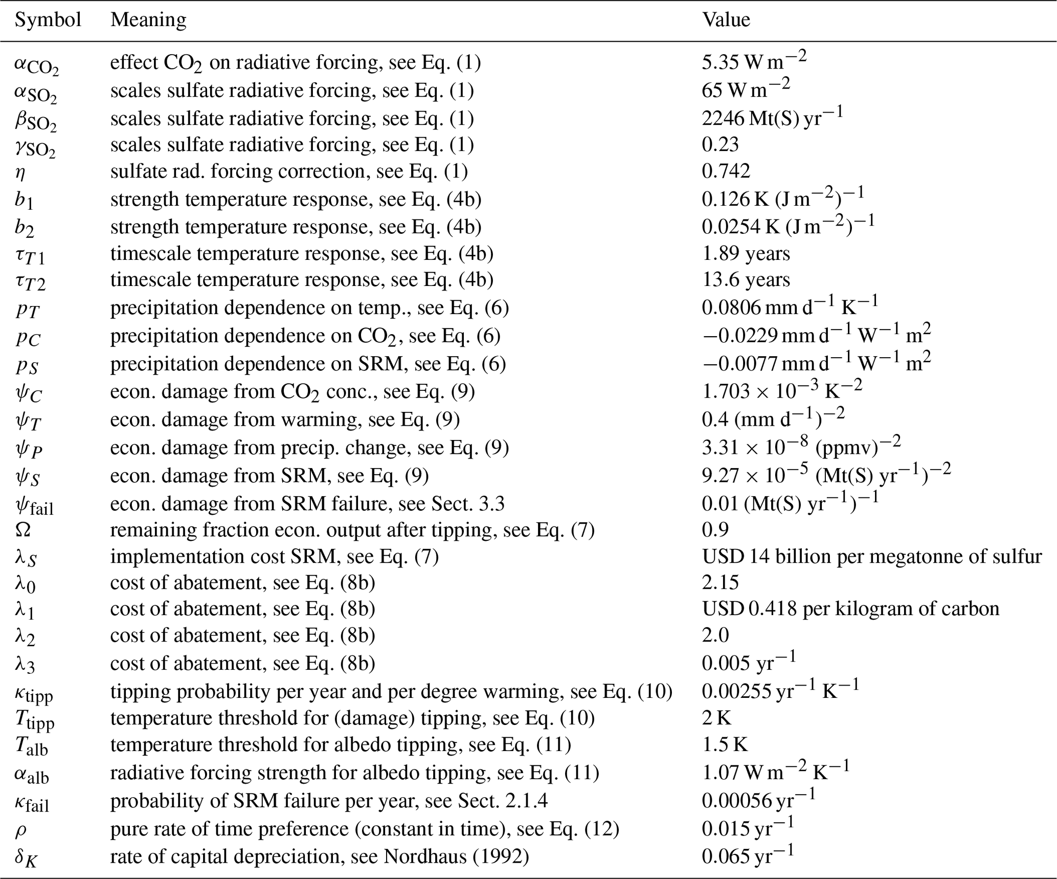
Our code is based on Cai et al. (2016), which in turn combines the 2013 version of DICE (Nordhaus, 1992, 2018) and the DSICE framework (Cai et al., 2012) for stochastic treatment of DICE. Here, we include SRM as an additional policy option (together with CO₂ abatement). To this end, we incorporate the cooling effect, implementation costs, and environmental damages of SRM into DSICE. A summary of the model parameters and their standard values is given in Table 1.

Table 1Model parameters of the GeoDICE model related to the representation of SRM. The carbon model parameters can be found in Table 5 of Joos et al. (2013), and others in DICE or DSICE (Cai et al., 2012).

Download Print Version | Download XLSX

2.1.3 The damage function and SRM costs

As in DICE (Nordhaus, 1992), the gross domestic product (GDP) $\stackrel{\mathrm{‾}}{Y}$ is diminished by climate-related damage and by expenditures for climate policy (CO₂ abatement and SRM implementation). Including these losses, we retain for the net output

$$\begin{array}{}\text{(7)}& Y=\mathrm{\Omega }{\displaystyle \frac{\mathrm{1}}{\mathrm{1}+D}}\mathrm{\Lambda }\stackrel{\mathrm{‾}}{Y}-{\mathit{\lambda }}_S{I}_S.\end{array}$$

Here, Ω describes damage due to tipping points (see Sect. 2.1.4). If tipping has occurred, then Ω=0.9 (reducing the economic output), otherwise Ω=1 (output not reduced). D≥0 describes non-tipping damage (discussed below). Λ is a factor describing the abatement costs (Λ<1 in case of abatement and Λ=1 in case of no abatement) taken over from DICE-2013 (Nordhaus and Boyer, 2000; Nordhaus, 2018):

$$\begin{array}{}\text{(8a)}& {\displaystyle }& {\displaystyle }\mathrm{\Lambda }\left(\mathit{\mu }\right)=\mathrm{1}-{\mathrm{\Lambda }}_{\mathrm{0}}\left(t\right){\mathit{\mu }}^{{\mathit{\lambda }}_{\mathrm{0}}},\text{(8b)}& {\displaystyle }& {\displaystyle }{\mathrm{\Lambda }}_{\mathrm{0}}\left(t\right)={\displaystyle \frac{{\mathit{\lambda }}_{\mathrm{1}}\mathit{\sigma }\left(t\right)}{{\mathit{\lambda }}_{\mathrm{2}}}}[{\mathit{\lambda }}_{\mathrm{2}}-\mathrm{1}+\exp (-{\mathit{\lambda }}_{\mathrm{3}}t\left)\right],\end{array}$$

where σ(t) is the carbon intensity (amount of carbon released per dollar production, in absence of abatement) and λ_i are constants. Since CO₂ emission is proportional to $\stackrel{\mathrm{‾}}{Y}$, so are abatement costs (the more economic output, the more CO₂ emissions and hence the higher the costs of eliminating a fraction, μ, of these emissions). λ_SI_S is the implementation cost of SRM, which we assume to be linear in the injection rate I_S and independent of $\stackrel{\mathrm{‾}}{Y}$. Two studies (McClellan et al., 2010; Moriyama et al., 2017) suggest that the costs for lifting gases to 20 km height are of the order of USD 2–10 billion per megatonne of injected gas. Taking an intermediate value of USD 7 billion per megatonne, and assuming that the gas used is SO₂ (which has twice the molecular weight of elementary S), this amounts to USD 14 billion per megatonne of sulfur. Note that H₂S would have a lower weight per mole of S, which might reduce transportation costs. However, H₂S is also more poisonous and thus potentially difficult to handle. To be conservative, we assumed the costlier solution.

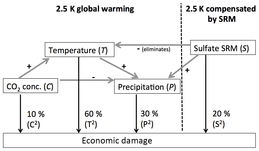
Figure 1Graphical representation of the damage function. The thin black arrows represent contributions to the damage function, while grey arrows depict how the climate variables influence each other (+ and − stand for increasing and decreasing effects, respectively, see Eqs. 4b and 6). The percentages for C, T, and P are based on the contributions of these variables for the standard case of 2.5 K warming in equilibrium and in absence of SRM. In this standard case, our damage equals that of the DSICE model (Cai et al., 2012). The sulfur injections that would be needed to offset 2.5 K warming cause a direct damage of 20 % of the standard damage function.

Download

While the original DICE model assumes that climate-induced damage D scales with the square of temperature change T² (i.e. D(T)=ψ₀T² with constant ψ₀), we keep the quadratic structure but split the damage function into three climate-related contributions and one contribution representing the damage inflicted by sulfate SRM (see Fig. 1):

$$\begin{array}{}\text{(9)}& D(T,P,C,I_S)={\mathit{\psi }}_T{T}^{\mathrm{2}}+{\mathit{\psi }}_P{P}^{\mathrm{2}}+{\mathit{\psi }}_C{C}^{\mathrm{2}}+{\mathit{\psi }}_S{I}_S^{\mathrm{2}},\end{array}$$

where T, P, and C are the changes (w.r.t. pre-industrial levels) in global mean temperature, global mean precipitation, and atmospheric CO₂ concentration, respectively, and I_S the sulfur injection rate in megatonnes of sulfur per year (Mt(S) yr⁻¹). Note that while SRM counteracts the effect of CO₂ on both temperature and precipitation, the relative influence of the forcing agents on both variables differs, so that it is not possible to compensate the warming and precipitation change at the same time. Both positive and negative precipitation changes, P, are considered damaging because both require ecosystems and humanity to adapt. An increase in atmospheric CO₂ may not be damaging in itself, or may even benefit plant growth (Ciais et al., 2013), but we consider C as a (rough) proxy for ocean acidification, which we do not model explicitly. The coefficients ψ (for values see Table 1) are chosen such that for the standard case of 2.5 K warming in equilibrium without SRM, our total damage equals that of the original DICE model, and the contributions by T, P, and C are 60 %, 30 %, and 10 %, respectively. The standard case was determined by running the climate module of GeoDICE to equilibrium with constant greenhouse-gas concentrations, such as to obtain T=2.5 K. Following Aengenheyster et al. (2018), and approximately in agreement with RCP (representative concentration pathway) scenarios, it was assumed that other forcing agents (other greenhouse gases and aerosols constituting F_other) contribute 14 % to the total radiative forcing. These other forcing agents are not assumed to cause direct damage. The damages associated with the annual sulfur injections needed to offset a warming of 2.5 K are assumed to equal 20 % of the standard case damage.

Previous studies (Heutel et al., 2016, 2018) likewise split the damage function, but without including residual climate change (P). Heutel et al. (2018) assume oceanic and atmospheric CO₂ to cause 10 % of the total damage each (20 % in total). However, atmospheric CO₂ is not known to cause substantial direct damage and may even be beneficial to plant growth (Ciais et al., 2013), while oceanic CO₂ leads to ocean acidification. As mentioned, we do not explicitly compute oceanic CO₂ but reduce total CO₂-related damage to 10 % because half of the total damage in Heutel et al. (2018) seems in fact small. The splitting between T and P is somewhat arbitrary, but is based on the rough assumption that, although precipitation changes can have a substantial impact, much of the damage is either determined by temperature (especially sea level rise, a major contributor) or at least strongly influenced by it (e.g. hurricanes), hence ψ_T>ψ_P. The damage related to SRM depends on the injection rate, not on the percentage of compensated greenhouse-gas forcing as was (somewhat unrealistically) assumed in earlier studies (Heutel et al., 2016, 2018). The choice of ψ_S is again somewhat arbitrary as virtually no data on the economic damage of SRM is available. However, our main conclusions are unaffected by the exact choice of the parameters ψ (see Sect. 3.5).

2.2 Optimisation and performance measures

As in DICE, we assume that all decisions are made by a single policy maker who aims to optimise the welfare of the (homogeneous) world population. As in DICE, welfare depends entirely on consumption. The economic output is spent on investment, I=rY, and global consumption, $Lc=Y-I$, where r is the saving rate and L and c are the world population and per capita consumption, respectively. We assume a fixed saving rate of r=22 %. The utility u (which can be thought of as the current happiness of the world population) depends on c: $u=L(c^{\mathrm{1}-\mathit{\gamma }}-\mathrm{1})/(\mathrm{1}-\mathit{\gamma })$ with γ=2 and the quantity to be maximised is the expectation value 𝔼(W) of the welfare W (the time-integrated discounted utility):

where t is (discrete) time and ρ the rate of pure time preference. The greater ρ, the less the far-future count towards W. The morally correct value of ρ has been fiercely discussed (Stern et al., 2007; Lilley, 2012; Ackerman, 2007). Here, we will not join the ethical debate on the correct value, but use the standard value of 1.5 % and perform a sensitivity study with ρ=0.5 (see Sect. 3.5).

The decision variables are the amount of CO₂ abatement μ (the fraction of CO₂ avoided) and the sulfur injection rate I_S. The model is integrated in yearly time steps, but the decision variables μ and I_S are changed only once a decade to save computational effort. The policy (sequence of values for μ and I_S) is optimised such as to maximise the expected welfare, 𝔼(W), over a time horizon until 2400, though the far future is heavily discounted. The optimisation is performed using dynamic programming (see Appendix). Once an optimal policy is found, it is evaluated by running an ensemble of 5000 members with this policy and Monte Carlo realisations of the stochastic elements (climate tipping and SRM failure). The best policy is the one yielding the highest expected welfare 𝔼(W). For easier comparison, we define a performance measure based on the improvement of W under policy π with respect to a no-action policy ($\mathit{\mu }=\mathrm{0},I_S=\mathrm{0}$):

where W_π, W₀, and W_AD are the expectation values over the Monte Carlo ensemble of the welfare associated with policy π, the no-action case, and the optimal policy for the deterministic abatement-only case (the policy that would be optimal if the decision maker may only use abatement and no climate tipping occurs), respectively. By construction, the relative performance is 100 % for abatement-only scenario in the deterministic case.

Although the objective for the optimisation is the expectation value of the welfare, it is also interesting to investigate the range of possible welfare outcomes, especially the worst-case (or at least relatively bad) scenario. Hence we present two additional performance measures based on the 10th and 90th percentiles of the welfare W_π. Similar to Eq. (13) we define ζ_X(π), the X-percentile relative performance of a policy π as

where W_π,X is the Xth percentile of the welfare (discounted cumulated utility) for policy π. Note that W_AD and W₀ are still the mean (i.e. not percentiles) welfare associated with the optimal policy for the deterministic abatement-only case, and the no-action case, respectively.

2.3 Scenarios

In Sect. 3.1–3.2 we first consider three stylised policy scenarios. The first is the abatement-only scenario in which the decision maker is allowed to use CO₂ abatement but no SRM. The second is SRM-only scenario in which the decision maker uses only SRM until an SRM failure occurs, after which only abatement may be used. This scenario represents a society which does not reduce CO₂ emissions but relies entirely on SRM (until it fails). The third is abatement+SRM scenario where the decision maker can use both abatement and SRM, unless SRM fails, after which only abatement is used. A no-policy scenario with neither abatement nor SRM serves as benchmark for performance comparison (see Eqs. 13 and 14). These three standard scenarios are first discussed in a deterministic setting (Sect. 3.1), i.e. in absence of climate tipping and SRM failure, before addressing them in the full model with uncertainty (Sect. 3.2).

While the previous stylised scenarios serve to isolate specific effects, we also present the realistic storyline (see Sect. 3.3), which allows for the fact that it may take time to develop SRM technology, generate a legal framework and public support, and evaluate associated risks. Also, all these processes may fail or the effectiveness of SRM might be found to be too low. Therefore we assume that SRM will become possible only in 2055 and only at 30 % probability. To be precise, at each time step until 2055, there is an equal probability that humanity discovers that SRM is impracticable. In the first decade where SRM is allowed, there is a 20 % probability of SRM failure, 10 % in the second decade, 5 % in the third decade, and 1 % per decade after that, i.e. after some decades of testing, failure becomes less likely. In this scenario, we also investigate the effect of damage in case of SRM failure (“termination shock”): SRM failure is accompanied by a one-time reduction of the GDP by a factor 1−ψ_failI_S, where I_S is the injection rate in megatonnes of sulfur per year (Mt(S) yr⁻¹) and ψ_fail is given in Table 1.

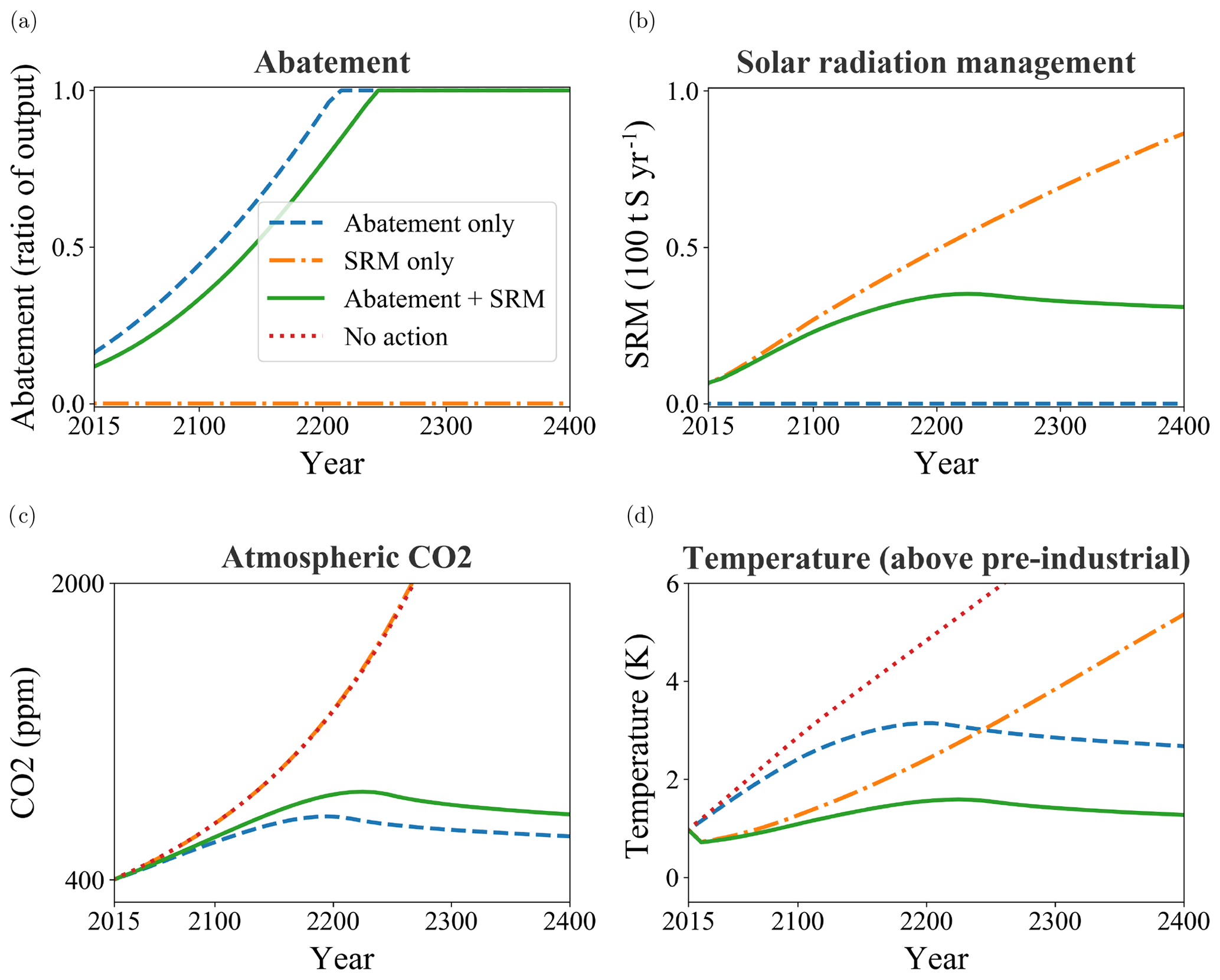
Figure 2Optimal policy and climate model results for the three stylised scenarios in the deterministic setting. (a) Abatement (fraction of CO₂ emissions avoided), (b) SRM (Mt(S) yr⁻¹), (c) atmospheric CO₂ concentration (ppmv), and (d) global mean temperature above pre-industrial temperature (K). The dashed blue line represents the abatement-only scenario, dashed-dotted orange line represents SRM-only scenario, solid green line represents abatement+SRM scenario, and dotted red line (only panel c and d) represents no climate action (i.e. neither abatement nor SRM).

Download

Table 2Comparison of policies in the deterministic setting (no tipping, no SRM failure). abatement-only scenario means that no SRM is used, SRM-only scenario means that no abatement is used (unless SRM fails see text), and in abatement+SRM scenario both are used. The performance ζ (see Eq. 13) is a measure of the increase in expected cumulated discounted utility w.r.t. the no-action scenario, and is normalised such as to yield 100 % for abatement-only scenario. The column “Peak SRM” contains the highest SRM values (in Mt(S) yr⁻¹) over all time steps. “Ab 50 %” and “Ab 99 %” show the year in which the abatement reaches 50 % and 99 %, respectively. SCC is the social cost of carbon in the first time step (measured in USD (in 2005) per tonne of carbon).

^* SRM does not peak but keeps increasing until the upper limit of 100 Mt(S) yr⁻¹. n/a means not applicable.

Download Print Version | Download XLSX

3.1 The deterministic case

As a reference, we first consider the deterministic case, i.e. without SRM failure and tipping points, in the three stylised scenarios (see Fig. 2 and Table 2). Allowing SRM in addition to abatement delays abatement by 2–3 decades, but does not replace it (Fig. 2a). CO₂ concentrations in abatement+SRM scenario (Fig. 2c) peak slightly later than in abatement-only scenario and reach higher values (875 ppmv instead of 741 ppmv). SRM helps to reduce global warming considerably: the global mean temperature change T peaks at 1.6 K for abatement+SRM scenario but at 3.1 K for abatement-only scenario (Fig. 2d). SRM slightly decreases towards the end of the simulation, when CO₂ concentration also goes down. This illustrates the potential use of SRM as a transition technology, especially under ambitious abatement: SRM can be used for a limited time in modest strength to cut off a warming overshoot.

In SRM-only scenario, CO₂ concentrations reach 2000 ppmv in 2260 and continue to increase (Fig. 2c). Note that currently known fossil fuel reserves are insufficient to generate this much carbon, but it is not impossible that fracking and newly discovered coal deposits will lead to sufficient fuel resources (Cassedy and Grossman, 2017). The temperature increase T continues to rise, reaching 5.4 K in 2400 (Fig. 2d), although it is lower than in the no-action case (neither SRM nor abatement). Due to the sub-linear increase in the radiative forcing with SRM, very high SO₂ injection rates would be needed to stabilise T with SRM-only scenario so that the damage related to sulfate injection outweighs the climate damages. Compared to SRM-only scenario, considerably less SRM is needed in abatement+SRM scenario, namely ≈35 Mt(S) yr⁻¹ (Fig. 2b; 3-4 Pinatubo eruptions per year), yet T remains much lower. This suggests that abatement is required in order to achieve long-term temperature stabilisation.

The relative performance ζ(π) for SRM-only and abatement+SRM scenarios becomes 186 % and 238 %, respectively (see Table 2). (By construction, ζ=100 % for abatement-only scenario in the deterministic setting.) The reason for the better performance of SRM-only scenario compared to abatement-only scenario is that SRM-only scenario yields lower temperatures and a higher utility in the first two centuries, which contribute most to the cumulative utility due to discounting. In addition, postponing damage is beneficial as it allows more time for accumulating capital.

3.2 The effect of uncertainties

Table 3Comparison of policies in the stochastic setting, i.e. including climate tipping and SRM failure. No-action case means that neither abatement nor SRM are used; other scenarios are explained in Sect. 2.3. The performance measures ζ, ζ₁₀, and ζ₉₀ are given in Eqs. (13) and (14). The columns “SRM fail” and “Tipping” show the probability that SRM failure or climate tipping occurs before 2415. The column “Peak SRM” contains the highest SRM value (in Mt(S) yr⁻¹) over all time steps and over all ensemble members. This corresponds to members in which no SRM failure or climate tipping occurred, at least before the time of the SRM peak. “Ab 50 %” and “Ab 99 %” show the year in which the abatement reaches 50 % and 99 %, respectively. SCC is the social cost of carbon in the first time step (measured in USD (in 2005) per tonne of carbon).

¹ SRM does not peak but keeps increasing until the upper limit of 100 Mt(S) yr⁻¹. ² Tipping can occur but the policy maker ignores this and chooses the policy which would be optimal in the deterministic (det.) case. n/a means not applicable.

Download Print Version | Download XLSX

Figure 3Tipping risk and policy in the stochastic setting (i.e. with tipping point and SRM failure). (a) cumulative probability of tipping for abatement-only scenario (blue dashed line), SRM-only scenario (yellow dash-dotted) and abatement+SRM scenario (green solid). (b–l) policy and climate response for the same scenarios (zoomed in on years 2015–2300 to enhance readability), namely abatement-only (d, g, j), SRM-only (b, e, h, k), and abatement+SRM (c, f, i, l) scenarios. Variables shown are SRM deployed (b, c); note the different y-axis scale), abatement fraction (d, e, f), atmospheric CO2 content in ppmv (g, h, i), and global mean temperature change (j, k, l); note the different y-axis scale). The thin blue lines represent a sample of individual ensemble members, the thick red line the ensemble mean, and the blue shaded area indicates the range of possible values in the whole ensemble. The dashed blue line depicts the results from the deterministic case (Fig. 2) for reference.

Download

Next we include the stochastic elements, temperature-induced tipping, and SRM failure, and determine again the optimal policies for each scenario, prior to evaluating the optimal policy by means of a Monte Carlo ensemble (see Sect. 2.2). In Fig. 3b–l, we plot the policy (abatement and SRM), carbon concentration, and temperature for the three stylised scenarios. The plots depict some sample paths of individual Monte Carlo runs (thin blue lines), the range of possible outcomes (shading) and the ensemble mean (red line). For comparison, the results from the deterministic case (compare Fig. 2) are also plotted (dashed blue lines).

In the abatement-only scenario, the danger of tipping initially leads to higher abatement (Fig. 3d) than in the deterministic case, although the temperature is not kept below the 2 K threshold (see Fig. 3j). If tipping occurs, the abatement decreases again as there is no further tipping point to be avoided. (This effect is caused by having a single tipping point which, once activated, does not react to system changes. Compare the Albedo tipping point in Sect. 3.4.) The relative performance is 105 % (see Table 3, row 3), i.e. it slightly improves when the decision maker takes tipping into account (compare Table 3, row 2). Recall that the reference scenario for W_AD uses the policy that would be optimal in absence of tipping, i.e. the policy maker ignores climate tipping.

In the abatement+SRM case, the optimal policy closely resembles the deterministic one if no SRM failure occurs (Fig. 3c, f). Without SRM failure, T stays below 2 K (Fig. 3l) and hence no tipping occurs. In case of an SRM failure, the temperature suddenly increases and abatement suddenly increases, as the decision maker now tries to limit the warming (and tipping risk) with only abatement. Note that such a sudden increase in abatement may not be feasible in reality. If climate tipping occurs, abatement is reduced again. Compared to abatement-only scenario, the abatement is delayed by 3–4 decades.

In the SRM-only scenario, the policy again resembles the deterministic case provided no SRM failure occurs and T is below 2 K (Fig. 3b). When T=2 K is reached, SRM increases sharply to reduce the tipping risk. As before, abatement strongly increases after SRM failure, but is reduced slightly if tipping occurs (Fig. 3e). SRM-only scenario has a performance of 181 %, much higher than abatement-only scenario. However, the chance of climate tipping by the year 2415 is considerably higher for SRM-only scenario (61.0 % vs. 37.8 % for abatement-only scenario, see Table 3). As in the deterministic setting, the reason is that initially SRM can control the global warming more effectively than abatement, while abatement is a long-term measure. Hence damage is postponed to the far future which is heavily discounted. The cumulative probability of tipping is lower for SRM-only scenario than for abatement-only scenario until 2350, when the situation reverses (Fig. 3a).

Compared to the deterministic cases, including uncertainty slightly reduces the difference in relative performance between abatement-only scenario and the scenarios using SRM (compare Table 3 vs. Table 2). There are two competing effects: the danger of tipping might favour using SRM, which reduces the tipping probability in the near future, while the possibility of SRM failure reduces the performance of SRM-based scenarios.

In abatement-only scenario, there is a high spread between the relative performance measures ζ, ζ₁₀, and ζ₉₀ compared to SRM-only and abatement+SRM scenarios. This is due to the fact that in most (>90 %) of the ensemble members, SRM keeps global warming below 2 K at least until ≈2200. Hence SRM postpones climate tipping into the far future (except in the few ensemble members with early SRM failure); for abatement-only scenario, tipping can occur as early as 2080. Early tipping greatly reduces the performance because it reduces the GDP for a long period of time and because it is less heavily discounted. For abatement+SRM scenario, only 6.2 % (i.e. <10 %) of the ensemble members show climate tipping, but they strongly affect the mean performance. This explains why, for this scenario, ζ<ζ₁₀.

Although DICE is too limited to give reliable absolute values of the social cost of carbon (SCC) (van den Bergh and Botzen, 2015), comparing scenarios gives qualitative insight into how SRM affects the SCC (Table 2 and Table 3). For abatement-only scenario, the SCC in 2015 is USD 35 per tonne of carbon (in 2005 USD) in the deterministic case and USD 41 per tonne of carbon when including tipping points. For abatement+SRM scenario, the SCC is USD 20 per tonne of carbon (both deterministic and stochastic): SRM lowers the SCC by partially compensating the damage caused by CO₂ emissions. For SRM-only scenario, the SCC is only slightly higher, namely USD 21 per tonne of carbon (deterministic) and USD 23 per tonne of carbon (stochastic) because SRM suppresses most climate damage in the near future, which is discounted least.

3.3 Realistic storyline

The previous scenarios were very stylised, in order to isolate the impact of SRM and stochastic elements. However, the actual situation is more complex: presently SRM is not available and we do not know whether it ever will be; yet we might want to decide now whether to pursue (research and development of) SRM. To address this question, we consider a “realistic storyline” scenario in which we assume that SRM will become possible only in 2055, and only at 30 % probability (in the decades before 2055, there is a certain probability each time step that SRM is declared infeasible, e.g. because scientists identify unacceptable environmental risks). We also assume that after 2055, the probability of SRM failure decreases in time, i.e. with ongoing testing, and allow for damage associated with a termination shock in case of SRM failure (see Sect. 2.3). Unlike (irreversible) climate tipping, the termination shock is a short-lived phenomenon and is stronger for extensive SRM.

In those ensemble members where SRM becomes available in 2055, it is used sparingly in the first time step because the probability of failure is still high and the decision maker wants to limit the termination shock. In later time steps, SRM is used only slightly less than in the abatement+SRM scenario, peaking at 31.4 % rather than 35 %. This difference mainly arises because the decision maker wants to reduce the termination shock: if the termination shock damage is omitted from the realistic storyline, SRM peaks at 34.7 %.

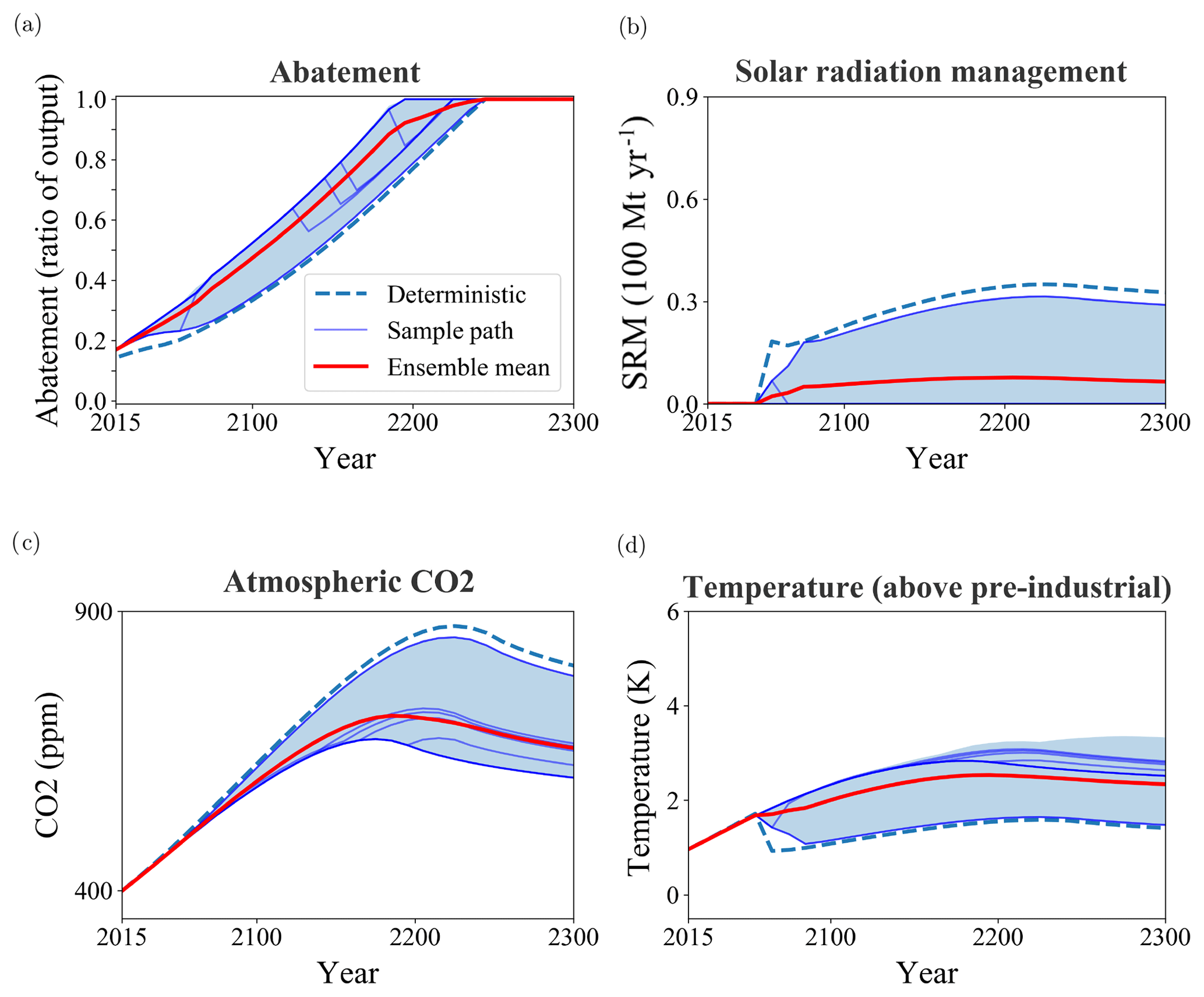
Figure 4Optimal policy and climate development for the realistic storyline scenario. (a) Abatement fraction, (b) SRM in 100 Mt(S) yr⁻¹, (c) atmospheric carbon concentration in ppmv, (d) global mean temperature change w.r.t. pre-industrial temperature. The thin blue lines represent a sample of individual ensemble members, the thick red line the ensemble mean, and the blue shaded area indicates the range of possible values in the whole ensemble. The dashed blue line depicts the results from a deterministic reference case in which SRM becomes available in 2055 certainly and neither SRM failure nor climate tipping occur.

Download

In the first time step (2015), when the decision maker assumes that SRM will become available with 30 % probability only, the abatement μ(2015)=0.17, only slightly less than in the abatement-only scenario where μ(2015)=0.18. For comparison, in a deterministic reference case in which SRM will be available from 2055 certainly, and no SRM failure or tipping occurs, μ(2015)=0.14 (see Fig. 4). As time progresses until 2055, the ensemble members diverge: if SRM is already banned, abatement increases, but if a time step has passed without a ban, the decision maker becomes more optimistic that SRM will become feasible and abatement becomes less ambitious. In ensemble members where SRM becomes available, 50 % abatement is reached 45 years later than in cases where SRM remains impossible. For current policy, however, the most important point is that in 2015 (“now”), a 30 % chance of SRM becoming available does not lead to significant reduction in optimal abatement.

On the other hand, the performance, ζ, of this scenario is 125 % (Table 3), significantly higher than for abatement-only scenario. The lowest 10th percentile performance, ζ₁₀, is very similar to the abatement-only scenario. In the realistic storyline, the low-performance members are those in which SRM never becomes available, and the policy (i.e. trajectory of abatement) in these runs is very similar to abatement-only scenario. However, ζ₉₀ is much higher for the realistic storyline than for abatement-only scenario. This measure is dominated by those members in which SRM becomes available. The total climate tipping risk for the realistic storyline is 30.1 % compared to 37.8 % in the abatement-only scenario. The SCC for the realistic storyline is USD 37 per tonne of carbon, 12 % lower than for abatement-only scenario.

These comparisons between the realistic storyline and abatement-only scenario indicate that the former performs better. This is because in those cases where SRM does become available, the welfare gain of climate policy is twice as high as in the abatement-only case. Therefore, a policy maker in 2015 should not dismiss SRM prematurely, but keep the option open (by encouraging research and development). If we are lucky and SRM works well, it can greatly enhance future welfare, whereas if it never becomes feasible we are not worse off than with abatement-only scenario. (Note, however, that we did not include the possibility of a large-scale SRM test with huge unexpected damage, but assumed careful well-designed research.) However, the prospect of possible future SRM should not lead to a significant reduction in abatement efforts at the current stage.

3.4 SRM as “climate insurance”

In the previous scenarios, SRM was used in a continuous way as a complement for abatement in order to further reduce global warming, especially when the warming was highest. Here we investigate under which circumstances it can be advisable to use SRM as an insurance, i.e. suddenly increase its use or even voluntarily delay using it at all.

First, we consider a situation in which SRM is very dangerous, and thus unattractive to use unless climate change is also very dangerous. This is achieved by assigning a very high, but one-time only, damage to SRM failure, namely reducing capital by a factor ${\mathrm{\Omega }}_K=I_S/(I_S+I_{S\mathrm{0}})$ in case of SRM failure. Here I_S is the injection rate in megatonnes of sulfur per year (Mt(S) yr⁻¹) and I_S0=5 Mt(S) yr⁻¹. This means that already at modest injection rates, SRM failure is assumed to cause substantial capital losses. In addition, we increase the likelihood of tipping failure by a factor of 4. Apart from these changes, the scenario is the same as the abatement+SRM scenario in Sect. 3.2. This scenario is not necessarily considered the most likely but serves as a proof of concept. The result is that SRM is not started until the tipping threshold T=2 K threatens to be reached (see Fig. 5a–c). When the threshold is reached, SRM is started and somewhat more SRM is applied than strictly necessary to keep below T+2 K. This is because in our parameterisation, damage levels off somewhat with increasing injection rate, i.e. if SRM is used at all, then a little extra does not make failure costs that much worse. The temperature increase is kept below T=2 K throughout, unless SRM fails. Compared to the standard abatement+SRM case, peak SRM is reduced to 27.6 Mt(S) yr⁻¹, i.e. by about 21 %, and 50 % abatement is reached in 2127, i.e. 12 years earlier. This experiment shows that the possibility of SRM causing high damage can cause a delay in its use until climate change also becomes very dangerous (tipping threshold reached).

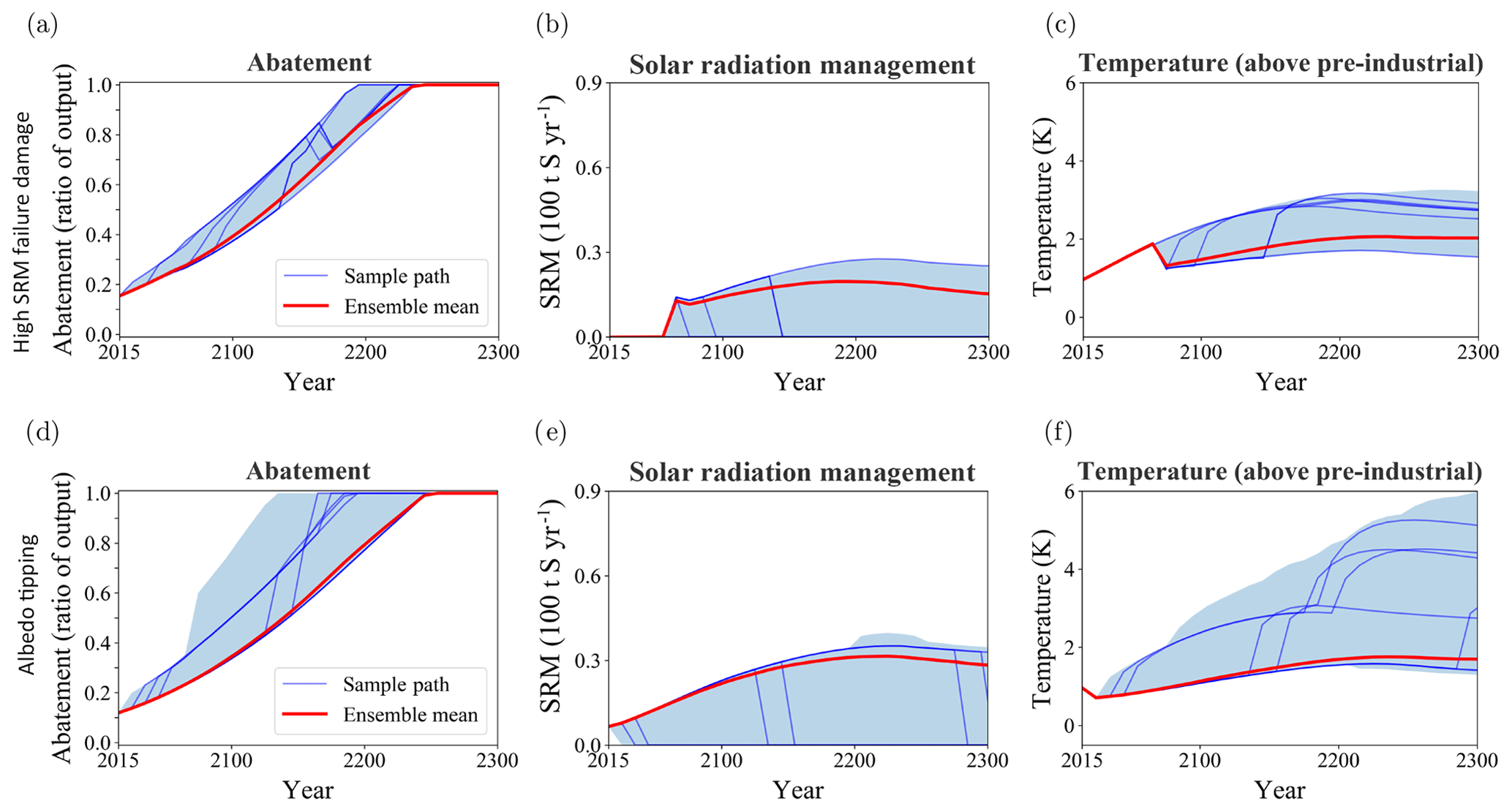
Figure 5Policy and temperature for the “SRM as insurance” scenarios (see Sect. 3.4). The top row shows the scenario with high damage in case of SRM failure, while the bottom row shows the scenario with an albedo tipping point. The left column (a, d) show abatement, the middle one (b, e) SRM, and the right (c, f) warming. The thin blue lines represent a sample of individual ensemble members, the thick red line the ensemble mean, and the blue shaded area indicates the range of possible values in the whole ensemble.

Download

Second, we replace the standard tipping point in abatement+SRM scenario by the “albedo” tipping point (see Sect. 2.1.4). It is found that if the policy maker can use SRM freely, they do not employ it to such a degree as to stay below $T=T_{\mathrm{alb}}=\mathrm{1.5}$ K but take the (small) chance of crossing the threshold. If this happens, they do increase SRM to counteract the albedo feedback (the bump after 2200 in Fig. 5e). Although the time step for determining policies is 10 years, the albedo feedback is weak enough that no runaway global warming occurs since, with SRM, T−T_alb and hence F_alb is small. This is why a modest increase suffices to suppress this effect. However, if SRM has failed, temperature is much higher than T_alb, increasing both the probability of albedo tipping and the radiative forcing strength if tipping occurs. As in the standard abatement+SRM scenario, the policy maker increases abatement in case of SRM failure to avoid the tipping point. However, if the albedo tipping occurs after SRM failure, the policy maker increases abatement yet again in order to limit the positive temperature feedback. Nonetheless, the albedo tipping can cause additional warming of more than 2 K. A positive climate feedback tipping point can thus lead to enhanced climate policy – SRM or abatement or both – after being triggered, in order to reduce its consequences.

3.5 Sensitivity analysis

Table 4Policy metrics of the sensitivity runs. “Abate 50 %” is the year in which abatement reaches 50 % (μ=0.5). “Peak SRM” (in Mt(S) yr⁻¹) is the highest SRM value of the ensemble (over all times and all members) and corresponds to those ensemble members without early SRM failure or climate tipping. “SCC” is the social cost of carbon in USD(2005) per tonne of carbon. All simulations were preformed in the stochastic settings and are either abatement-only scenario or abatement+SRM scenario (abbreviated here as Ab.+SRM). The first two cases, labelled “standard”, are repeated from Table 3 for convenience. The sensitivity runs correspond to those discussed in Sect. 3.5. n/a means not applicable.

Download Print Version | Download XLSX

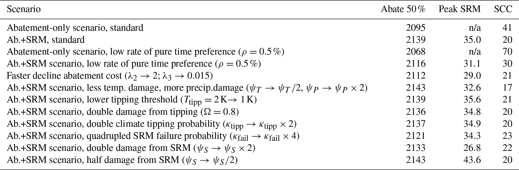
The results of our model substantially depend on the rate of time preference ρ (see Sect. 2.2). In abatement-only scenario, reducing ρ from the standard value of 1.5 % to a lower value of 0.5 % will lead to stronger abatement: 50 % abatement is reached 27 years earlier (see Table 4). This is expected as a lower rate of time preference means that the decision maker gives more weight to the welfare of future generations and is more willing to sacrifice present consumption to reduce climate change. The SCC rises from USD 41 to USD 70 per tonne of carbon. Interestingly, abatement also increases in the abatement+SRM scenario (50 % abatement is reached 23 years earlier) when reducing ρ to 0.5 %, while the peak SRM (definition: see Table 3) decreases by about 11 %. In other words, a decision maker who cares strongly about the future will choose to reduce CO₂ emissions rather than forcing future generations to rely on SRM, which causes damages and might fail. The SCC rises from USD 20 to USD 30 per tonne of carbon.

A potentially important limitation of DICE is that abatement costs are exogenous, whereas in reality one would expect costs to decline with growing employment (learning by doing). While fully exploring learning by doing is outside the scope of this study, we estimate the sensitivity to abatement costs in a simulation wherein abatement costs decrease more quickly in time and reach a lower value for t→∞. This is done by putting λ₂=1.5 and λ₃=0.015 in Eq. (8b), which lowers abatement cost by a factor of about 0.6 after 70 years compared to the standard scenario. The resulting policy shows a faster abatement by about 30 years, leading to a lower peak in atmospheric carbon (745 ppm instead of 870 ppm). Peak SRM is reduced to 29 Mt(S) yr⁻¹, as less SRM is needed if carbon concentrations are lower. Thus the development of abatement cost can significantly affect the need for SRM.

The distribution of the damages between the two major contributors, namely warming and residual climate change, was chosen rather arbitrarily. However, halving ψ_T (warming contribution) and doubling ψ_P (residual contribution) does not qualitatively affect our results. A 50 % abatement is reached 4 years later in the abatement+SRM scenario, and SRM peaks at 32.6 Mt(S) yr⁻¹ instead of 35.0 Mt(S) yr⁻¹, i.e. the optimal policy still combines a similar abatement with modest SRM. The SCC drops from USD 20 to USD 17 per tonne of carbon. Lowering the tipping threshold from 2 to 1 K leads to a 2 % increase in peak SRM, while not affecting abatement. Doubling the damages associated with climate tipping ($\mathrm{\Omega }=\mathrm{0.9}\to \mathrm{\Omega }=\mathrm{0.8}$) only accelerates 50 % abatement by 3 years in the abatement+SRM case and the SCC remains at USD 20 per tonne of carbon. Doubling the likelihood of climate tipping (κ_tipp) accelerates 50 % abatement by 2 years and likewise does not affect SCC. Increasing the failure probability of SRM (κ_fail) by a factor of 4, i.e. such that SRM failure occurs in 80 % of the ensemble members rather than 20 %, increases the SCC only by 15 % in the abatement+SRM scenario, i.e. from USD 20 to USD 23 per tonne of carbon. The reason is that the likelihood of SRM failure in the first decades, which are least discounted, is still fairly small. The peak SRM is reduced only by 2 %: as long as SRM is available, it is used despite high failure probability. A 50 % abatement is reached in 2121, rather than 2138, in the ensemble mean. Doubling the damage associated with SRM (i.e. doubling ψ_S) accelerates 50 % abatement by 6 years and the SCC rises from USD 20 to USD 22 per tonne of carbon. The peak SRM is reduced by about 23 %, to 26.8 Mt(S) yr⁻¹. Likewise, halving ψ_S increases peak abatement by 25 %. Hence even if SRM is twice (or half) as damaging as assumed in the standard case, the optimal policy still employs modest SRM as a complement to abatement.

To summarise, changes in the damage function and/or likelihood of stochastic events do not qualitatively affect the optimal policy in the abatement+SRM scenario, which consists of a combination of reasonably high abatement (delayed by a few decades w.r.t. abatement-only scenario in the standard settings) and modest SRM.