the Creative Commons Attribution 4.0 License.
the Creative Commons Attribution 4.0 License.
 | 27 Jun 2019
Millennium-length precipitation reconstruction over south-eastern Asia: a pseudo-proxy approach
Stefanie Talento
Lea Schneider
Johannes Werner
Jürg Luterbacher
Quantifying precipitation variability beyond the instrumental period is essential for putting current and future fluctuations into long-term perspective and providing a test bed for evaluating climate simulations. For south-eastern Asia such quantifications are scarce and millennium-long attempts are still missing. In this study we take a pseudo-proxy approach to evaluate the potential for generating summer precipitation reconstructions over south-eastern Asia during the past millennium. The ability of a series of novel Bayesian approaches to generate reconstructions at either annual or decadal resolutions and under diverse scenarios of pseudo-proxy records' noise is analysed and compared to the classic analogue method.
We find that for all the algorithms and resolutions a high density of pseudo-proxy information is a necessary but not sufficient condition for a successful reconstruction. Among the selected algorithms, the Bayesian techniques perform generally better than the analogue method, the difference in abilities being highest over the semi-arid areas and in the decadal-resolution framework. The superiority of the Bayesian schemes indicates that directly modelling the space and time precipitation field variability is more appropriate than just relying on a pool of observational-based analogues in which certain precipitation regimes might be absent. Using a pseudo-proxy network with locations and noise levels similar to the ones found in the real world, we conclude that performing a millennium-long precipitation reconstruction over south-eastern Asia is feasible as the Bayesian schemes provide skilful results over most of the target area.


Earth's climate varies in all spatial and temporal timescales, as it is forced by either natural or anthropic factors. To understand the dynamics of such variability, the analysis of the available instrumental information is an essential tool. However, the time coverage of the instrumental records is rather short and, therefore, information from climate archives (natural and documentary) going back centuries is important to put current and future changes into a long-term perspective and to serve as a validation terrain for model simulations with the ultimate goal of understanding the underlying physical mechanisms.
South-eastern Asian societies and economies are heavily dependent on the summer rainfall (monsoon-dominated) as a freshwater resource; thus, it is important to investigate how these precipitation patterns have varied in the past to provide a useful guide for the climate response to future changes. Previous hydro climate field reconstructions (CFRs) over Asia revealed a substantial mismatch between modelled and reconstructed precipitation patterns (Shi et al., 2017) and the spatial variability of large-scale droughts during the Little Ice Age (Cook et al., 2010; S. Feng et al., 2013). While these studies covered the last 500–700 years, a gridded hydroclimate product going beyond Medieval times at a spatio-temporal high resolution is still missing. Whether such a long and highly resolved reconstruction is possible given data and methodologies available nowadays is the subject of this paper.
Reconstructing the temporal evolution of climatic variables in the space domain (CFR) based on the information from a sparse network of proxies and partially overlapping instrumental data is a complex mathematical problem. First of all, the proxy data used for generating reconstructions display a set of characteristics that make their use challenging: their distribution in space and time is heterogeneous with fewer records further back in time; different proxy archives have different temporal resolutions and possibly include dating uncertainties; proxy data might reflect different climate variables (temperature, precipitation, sea-level changes, pH, seawater temperature, water mass circulation, etc.), recording climate conditions at different times of the year, and these data contain non-climatic information (usually referred to as non-climatic noise). Second, the overlap with instrumental observations is commonly short, limiting opportunities for statistical learning and further validation. Third, and in contrast to average climate reconstructions, CFRs require the spatial scale-up of the available information, therefore implying the need for strategic inferring of the missing values in the target climate field, even in locations where no data might be input. Finally, as the amount of paleoclimatic information becomes smaller back in time, it is virtually impossible to have an independent proxy data set to properly validate the output reconstruction. A common approach to overcome this shortcoming and have a proper validation stage is to use a pseudo-reality. The process of using a global climate model (GCM) simulation to assess the ability of a reconstruction technique is known as a pseudo-proxy experiment (PPE; Smerdon, 2012; Mann and Rutherford, 2002). In a PPE, simulated data are modified to mimic real-world proxies and instrumental observations (called pseudo-proxy and pseudo-instrumental data sets), and the reconstruction algorithms are applied. The reconstruction results are then compared with the available simulated target field, giving an estimation of the skill of the method in real-world applications.
There are several ways to perform a CFR (see Luterbacher and Zorita, 2018, for a review). The classical approach is through a multivariate regression perspective: a statistical relationship between proxy and instrumental data is inferred from the overlapping (calibration) period and then, assuming stationarity of this relationship, the missing instrumental values are predicted or reconstructed back through time. Some of the most common techniques for climate reconstructions included in this category are regularised expectation–maximisation (RegEM, Schneider, 2001), canonical correlation analysis (CCA; Smerdon et al., 2010), Markov random fields (Guillot et al., 2015) and the analogue method (Franke et al., 2011). The performance of these methods strongly depends on the length of the instrumental data. If the overlapping period between proxy and instrumental data is short, in comparison with the number of spatial locations considered, the estimation of the covariance matrix is uncertain and the matrix inversion process is numerically unstable, leading to poor performance when presented with new data out of the learning sample.
Another strategy to perform a CFR, more novel as it has only recently been applied in paleoclimatology, is the Bayesian approach (e.g. Tingley and Huybers, 2010, 2013; Werner et al., 2013, 2018; Luterbacher et al., 2016; Zhang et al., 2018). The Bayesian strategy is probabilistic, incorporates information about the climate–proxy connection as constraints on the reconstruction problem and has the benefit of providing more comprehensive uncertainty estimates for the derived reconstructions. Robust comparisons between established methods and the emerging efforts (Werner et al., 2013; Nilsen et al., 2018) underpin the benefits and justify further application of the computationally more expensive method. So far, most of the paleoclimatic applications of this methodology involve temperature reconstructions. Efforts to apply this probabilistic framework to the more complex and highly variable hydroclimate are only in the initial stages, but the advantages of the methodology over more classical approaches are auspicious.
Gómez-Navarro et al. (2015) used a PPE approach to assess the skill of several statistical techniques (classical regression methods and Bayesian) in reconstructing the precipitation of the past 2 millennia over continental Europe. The authors find that none of the schemes shows better performance than the others and that precipitation reconstructions over Europe are only possible given a spatially dense and uniformly distributed network of proxies, as the accuracy strongly deteriorates with distance to the proxy sites.
In this study we propose to evaluate, via PPE, the potential to generate a last-millennium summer precipitation reconstruction for south-eastern Asia. We use three CFR techniques: Bayesian hierarchical modelling (BHM), BHM coupled with clustering processes (with two different numbers of clusters), and the analogue method. For each of the schemes we perform two reconstructions: one at annual and one at decadal resolution. In addition, the influence of the noise level in pseudo-proxies on the final reconstruction is evaluated.
This is the first time that a BHM approach is applied to the hydroclimate of Asia, and its coupling with clustering techniques is a methodological advance, configuring an innovation in the field. The systematic evaluation of the skill of these probabilistic methods, and the comparison with the more classical and well-established analogue technique, is a necessary step to learning about the precipitation variability and the opportunities for or obstacles to generating long-range informed guesses about it. The PPE exercise is a fundamental validation step, essential for selecting the most appropriate method to improve real-world reconstructions and, finally, deriving a new and not previously attempted gridded product of south-eastern Asia summer precipitation during the last 1000 years. In this work only summer precipitation is targeted as the pseudo-proxy network selected is based on real-world indicators of summer hydroclimatic variations (see Sect. 2.2).
The paper is organised as follows. In Sect. 2 we present the data and methodology and describe in detail the three reconstruction techniques, as well as the skill scores used for quality evaluation. Section 3 is devoted to the results and discussions: we evaluate the skill of each of the reconstruction methods, at both annual and decadal resolution, and investigate the role of the pseudo-proxy noise. Finally, in Sect. 4 we present conclusions and a short outlook.
2.1 Model
As a virtual reality setup for our study we use one full-forcing simulation (run 001) of the Community Earth System Model (CESM) from the Last Millennium Ensemble (LME) project (Otto-Bliesner et al., 2016). The simulation is performed with a horizontal resolution of ∼2∘ (∼1∘) in the atmosphere and land (ocean and ice) components. The CESM is forced with reconstructions of the transient evolution of solar intensity, volcanic emissions, greenhouse gases, aerosols, land use conditions and orbital parameters, all together, for the period 850–2005. The target variable to reconstruct is June–July–August (JJA) precipitation over continental south-eastern Asia, here defined as all continental grid points in the domain Equator–50∘ N 72.5–127.5∘ E. Given the model resolution, this implies that the reconstruction is attempted over 366 grid points.
Figure 1 depicts the JJA mean precipitation in the run used in this paper, considering only the last 100 years of simulation (period 1906–2005). Historical simulations with the CESM show a reasonable performance in reproducing summer precipitation over continental Asia: the simulated JJA precipitation is generally in agreement with observations, although a false rainfall centre over the eastern Qinghai–Tibetan Plateau is generated in these simulations (Wang et al., 2015).
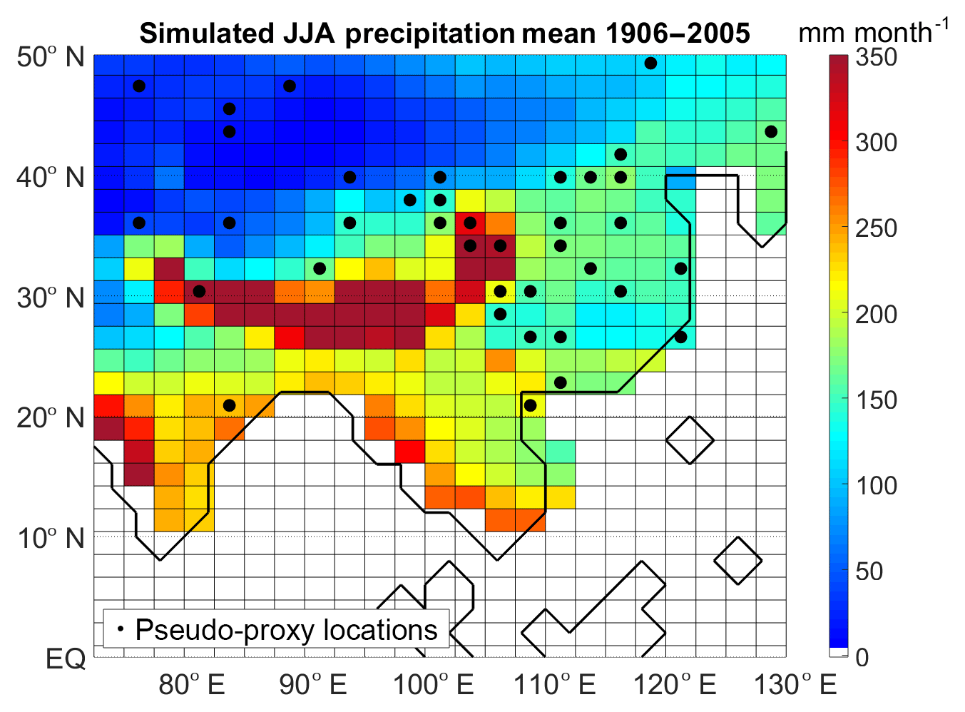
Figure 1Simulated mean JJA precipitation (millimetres per month) during the instrumental period (years 1906–2005) over continental Asia. Black dots: pseudo-proxy network.
2.2 Proxy data locations
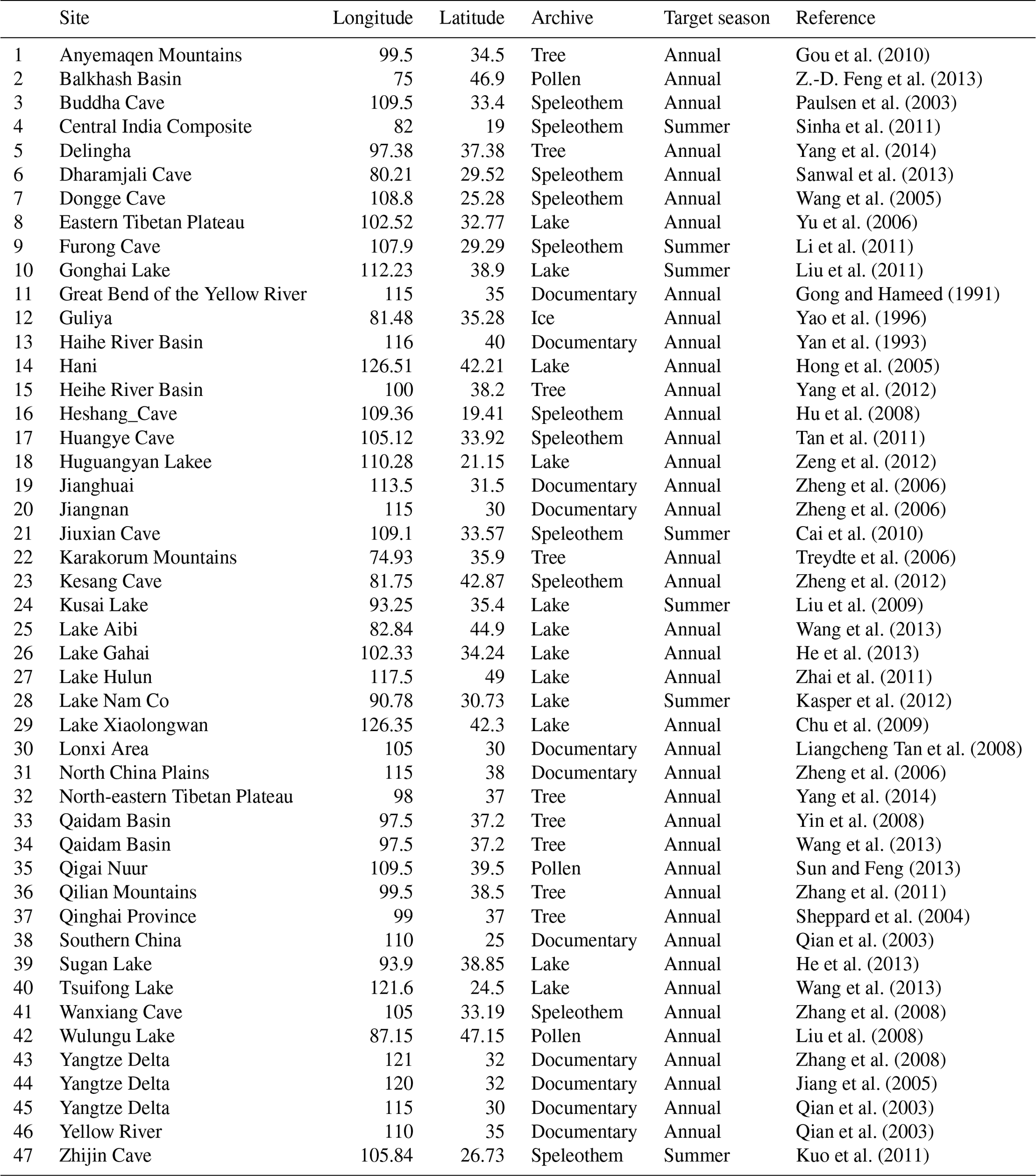
For this study we select the locations of 47 real-world precipitation-/drought-sensitive proxies in the target domain that span the last millennium. The locations of tree ring, speleothem, lake sediment and ice core sites as well as of some documentary data are mainly derived from the networks used in Chen et al. (2015) and Ljungqvist et al. (2016) (Table 1). The criteria for the selection of records were millennium-long (with start date before 1000 CE), at least two values per century, terrestrial, published in the peer-reviewed literature, and described as an indicator of local variations in hydroclimate.
Table 1List of the real-world proxy records used to select the locations of the pseudo-proxy network.
2.3 Design of the PPEs
For the design of the PPEs we build two data networks: a pseudo-proxy one and a pseudo-instrumental one. The pseudo-proxy network is based on the locations of the real-world hydroclimate proxies listed in Table 1. As some of these 47 records are in close proximity, this translates into having 38 different model grid points (about 10 % of the total grid points in the study region). The selected locations are not evenly distributed across south-eastern Asia: the highest concentrations are found over eastern China and over the dry lands in the north-west of the study region (Fig. 1). There are neither pseudo-proxy sites southward of 20∘ N nor over Mongolia and the Himalayas. To emulate real proxies, we consider the modelled precipitation time series spanning the complete period of the simulation (1156 years, either with annual or decadal resolution) at each of the 38 selected sites and contaminate them by the addition of noise. We select four different levels of additive Gaussian white noise, corresponding to null, low, medium, and high levels of noise. The selected noise levels are such that the correlations between the original and contaminated time series are 1, 0.7, 0.5, and 0.3, respectively. A correlation equal to 1 implies an idealised situation of perfect proxies to study the representativeness of our spatial sampling. A correlation of 0.7 represents an optimistic situation, but is still realistic: for example, Shi et al. (2014) find correlations of up to 0.7 with a tree-based reconstruction of the South Asian Summer Monsoon Index. A correlation of 0.5 between the proxy series and precipitation corresponds to a medium-level noise, and could be regarded as the average situation with real proxies (examples for Asia: He et al., 2018; Liu et al., 2013). A correlation of 0.3 represents a high-noise setting, which is still rather common in real-world proxies (e.g. Jones et al., 2009).
For the pseudo-instrumental network we consider all the locations for which a reconstruction is targeted: 366 model grid points in south-eastern Asia. For each of these locations, we take the modelled precipitation time series for the last 100 years of simulation (at either annual or decadal resolution) and add a small Gaussian noise to represent the instrumental errors present in real precipitation measurements. The added noise is such that, at each location, the correlation between the original and contaminated time series is 0.95.
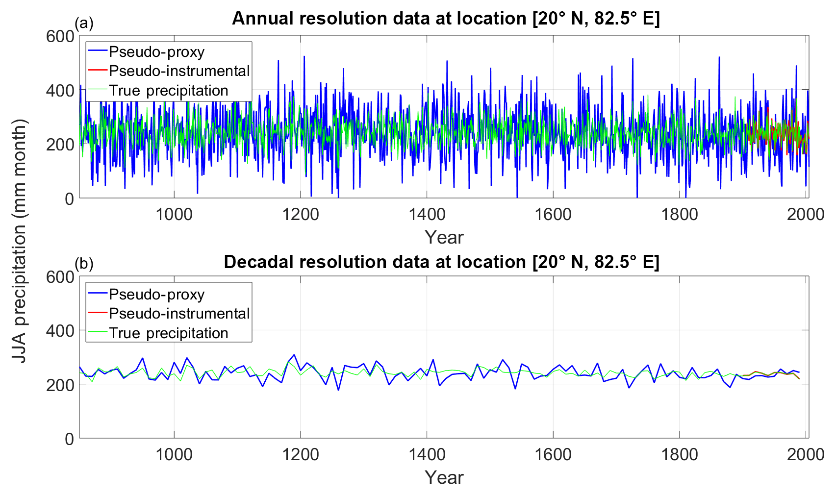
Figure 2Example of pseudo-proxy, pseudo-instrumental and true precipitation time series at location [20∘ N, 82.5∘ E]. (a) Annually resolved data. (b) Decadally resolved data.
As an example, Fig. 2 shows the simulated precipitation time series at location [20∘ N, 82.5∘ E] (eastern India) together with the associated pseudo-proxy and instrumental time series, both at annual and decadal resolution, for the case of medium-noise level (corresponding to a 0.5 correlation with the target precipitation). At annual resolution, the simulated mean JJA precipitation at this site is 241 mm per month, with a standard deviation of 48 mm per month. No statistically significant changes are found either in mean or variance. The maximum (minimum) summer precipitation at this location is 423 (87) mm per month and occurred in the year 1022 (1208) of the simulation, respectively. At decadal resolution, the standard deviation is reduced to 14 mm per month and the maximum (minimum) precipitation value is 283 (208) mm per month, occurring at the period 1180–1189 (870–879).
2.4 Reconstruction techniques
In the following subsections we describe in detail each of the three reconstruction techniques used in this paper.
2.4.1 Bayesian hierarchical modelling (BHM)
In the BHM technique a hierarchy of parametric stochastic models is used to describe the relationship between climate, instrumental and proxy data. The model parameters are estimated using the available data, through Bayes' rule. The hierarchy consists of three basic components. First, in the process level, a stochastic model describing the time evolution of the climate variable is selected. Second, in the data level, stochastic relationships between the instrumental and proxy data and the climate variable are developed. Finally, a level of prior information about the parameters involved in the other two components of the hierarchy is coupled. Here we use the BHM algorithm named the Bayesian Algorithm for Reconstructing Climate Anomalies in Space and Time (BARCAST), developed by Tingley and Huybers (2010). In the following, we specify the assumptions and equations for each of the levels in the model hierarchy.
Process level
The process level describes the evolution of the true climatic field as a multivariate autoregressive process of order 1, AR(1),with spatially correlated innovations.
The evolution of the true precipitation, sampled at a finite number of spatial locations, is assumed to follow a first-order autoregressive process:
where Prt is the vector consisting of the true precipitation values in all the locations at time step t, μ is the mean of the process, and α is the AR(1) coefficient. Note that the coefficients μ and α are the same for all the locations. To account for different precipitation means at each location the following procedure is followed: first, the time series are standardised; second, the BHM is applied; finally, the outputs are inversely de-standardised. The standardisation is performed using the sample mean and standard deviation from the pseudo-instrumental time series. The innovations ϵPr, t, accounting for the interannual or interdecadal variability, are assumed to be independent and identically distributed (iid) normal draws with an exponentially decaying spatial structure:
where |xi−xj| is the distance between the locations ith and jth of the precipitation vector, ϕ is the range parameter (1∕ϕ being the e-folding distance) and σ is the partial sill of the spatial covariance matrix (spatial persistence, homogeneous in space).
The temporal model within BARCAST allows the estimations of the field at a certain temporal step to be influenced by the information in the previous time step. The assumed covariance matrix structure is supposed constant in time and follows an exponentially decaying pattern with distance. Note that, by assuming this structure, if two distant locations have well-correlated precipitation time series, this will not be well represented by the BARCAST model assumed. The method parameterises the spatial covariance matrix with two unknown parameters: the covariance at null distance (σ) and the exponential decay rate with distance (ϕ).
The model assumes that the climatic variable, precipitation, follows a Gaussian distribution. Although this might not be the case, especially for arid regions, the simulated JJA precipitation in the area of study can be taken to reasonably follow this assumption: for the pseudo-proxy selected locations, 63 % of the time series (considering the instrumental period) pass the Kologorov–Smirnov test for normality at a 95 % confidence level (Fig. A1). Despite the Gaussian conditions not being met in all the grid points, the model is still valid, although it might not be the most optimal fit at these locations.
Figure 3 shows the correlation decay with distance for the simulated JJA precipitation for different latitudinal bands. For annual data (Fig. 3a), the correlation between precipitation time series in consecutive grid points is usually high, around 0.8. With few exceptions, the simulated precipitation follows an exponentially decaying pattern with distance, with points located further away than 600 km showing no significant correlation. Therefore, we take the exponentially decaying spatial structure of the covariance matrix in BARCAST to be a reasonable assumption for the model. For decadal data (Fig. 3b), the correlation behaviours are not uniform with respect to the latitudinal bands. For some of the latitudes the plot follows an exponentially decaying shape, and for others it additionally shows a teleconnection pattern (notably the northern-most 44–48∘ N latitude band).

Figure 3Correlation of simulated JJA precipitation time series across different latitudinal bands versus distance. Only the instrumental period (years 1906–2005) and the grid points in continental Asia are considered for the calculation. (a) Annual-resolution data. (b) Decadal-resolution data. Dashed horizontal lines indicate the thresholds of statistical significance at a 95 % confidence level according to the Student's t-test. For this plot, all grid points in the same latitude band are grouped together and then one-to-one correlations are calculated between members of the same group.
Data level
The data level specifies the relationship between the measurements (both proxy and instrumental) and the true field values.
The instrumental observations at each time are assumed to be noisy variations of the true precipitation field:
The noise terms are assumed to be iid multivariate normal draws , while HInst, t is a diagonal matrix with a 1 in position (i, i) if an instrumental observation is available at the ith location, and a 0 otherwise.
The proxy observations are assumed to follow an unknown statistically linear relationship with the true precipitation at each location:
Again, the HProx, t is a diagonal matrix with ones only for the locations with proxy observations, and the noise terms are iid normal draws: .
Prior level
To close the scheme, prior distributions must be specified for the eight scalar parameters and the initial climate field (i.e. at the first time step). We use the same priors as Tingley and Huybers (2010) and select prior distributions that are sufficiently diffuse to not have any important influence on the posterior distributions.
Using Bayes' rule the posterior distribution of each of the unknown variables can be calculated. Samples are drawn from these posterior distributions using a Gibbs sampler, with a Metropolis step (Gelman et al., 2003) to update ϕ, the spatial range parameter. The output of the Bayesian algorithm is not a unique reconstruction, but an ensemble of 1200 equally probable draws, all of them consistent with the model equations.
2.4.2 Bayesian hierarchical modelling coupled to clustering
Here we propose to couple the BHM with a clustering algorithm. The aim of the clustering step is to segregate south-eastern Asia into several clusters, according to similarities in the precipitation regimes during the pseudo-instrumental period. After the clustering, the BHM code is run within each cluster in an independent manner. Finally, all the results are merged together to produce the entire spatial reconstruction over the post-850 period. The idea behind the clustering step is to reduce the complexity of the problem to be presented to the BHM algorithm, as after clustering the code does not have to deal with extreme differences in precipitation regimes (as dipole patterns at mountain ranges) and a large number of grid cells.
We use a hierarchical agglomerative clustering technique. Each observation starts in its own cluster and pairs of clusters are agglomerated as one moves up in the hierarchy (Izenman, 2008). We select a complete-linking strategy: the distance between sets of observations is defined as the maximum of the pairwise distances between the observations in each of the sets. First, the method groups together the two closest observations, according to the selected distance, creating a cluster of two observations. Then, the sets whose distance is minimum are agglomerated together, iteratively repeating the process.
Here, the elements to cluster together are the different grid points in south-eastern Asia. The input variables for the method are the pseudo-instrumental precipitation time series at each of these locations. The distance between two points is defined as 1 minus the correlation between the pseudo-instrumental precipitation time series at these locations (points highly correlated display a small distance). In this way, the method groups together points whose pseudo-instrumental precipitation time series are highly correlated. We should note that the clustering algorithm does not require any expert knowledge as it is a fully unsupervised machine learning technique. This characteristic makes it easy to apply as a pre-BHM stage in any other context or area of study.
For both the annual and decadal reconstructions we select two cases: clustering into 5 and into 10 groups (note that the clusters might be different when using the annual/decadal information; see Fig. A2). We term the reconstructions in this category BHM+5Clusters and BHM+10Clusters. The criteria for the selection of the number of clusters were that most of the clusters should include pseudo-proxy locations (if a cluster does not include pseudo-proxy information, the BHM scheme only uses instrumental-period data). While this condition is met without problems for 5 clusters, with the 10-cluster division (in both the annual and decadal cases), one of the clusters is disjunct with the pseudo-proxy network. As a consequence, a higher number of clustering divisions was not attempted.
2.4.3 Analogue method
The analogue method is a learning technique first introduced by Lorenz (1969) for weather forecasting. The technique uses predictors to determine the value of the target variable, based on the statistical relationship between them in a learning set: the so-called pool of possible analogues. The method can also be applied to produce a CFR. In our study and for each time step (year or decade), the predictor variables are the proxy records (38 predictors) and the target variable is the complete precipitation field at the given time step. For the annually resolved reconstruction the learning set consists of the precipitation fields at each of the years in the instrumental period, i.e. all the time steps in which we simultaneously have the information about proxy and target. For the decadally resolved reconstruction, the learning set consists of the mean precipitation field in each possible 10-year period during the instrumental era.
The reconstruction of the precipitation field at time step t is obtained as follows. First, a distance between time steps is defined. Let ti be a time step included in the pool (instrumental period). Then, the distance between t and ti is, in this paper, defined as the Euclidean distance between the vectors of proxy data at times t and ti:
where Prox(lj,t) is the value of the proxy at location lj and time t. Locations are all the proxy locations (K=38). Second, the time steps in the pool are ordered according to their distance from t. Third, the N closest time steps are selected from the pool and are termed analogues: . Finally, the precipitation reconstruction for time t is the mean of the precipitation field in the N analogues:
N can be any value between 1 and the total number of elements in the pool of analogues. On the one hand, for annual (decadal) reconstructions, using N=1 will imply having a reconstruction identical to just 1 year (10-year mean) of the instrumental period and, therefore, particularities of this year (10-year period) might be involved. On the other hand, using the maximal N implies just giving as reconstruction the mean during the instrumental period, which eliminates all the inter-annual or inter-decadal variability. In this paper we select as N intermediate values, considering N approximately equal to 20 % of the number of possible analogues. Experiments using values of N between 15 % and 40 % of the number of possible analogues were performed and the results are not significantly different to the ones selected to be displayed here (not shown).
Note that in this paper we use the analogue method in its classical version (obtaining the pool of analogues from the observational data set) and not in combination with the use of a GCM to draw the analogue cases from.
2.5 Skill metrics
To evaluate the performance of the CFR methodologies, we compare the reconstruction with the true precipitation field. We select three different skill metrics. The first skill metric, the correlation coefficient, evaluates the ability of the reconstruction to reproduce the temporal evolution of the target. At each grid point, we calculate the Pearson correlation between the reconstruction and the true precipitation time series, considering the whole reconstruction period. As for the Bayesian algorithms, we have an ensemble of reconstructions: we first calculate the correlation of each of these ensembles with the true precipitation and, finally, we show the mean of these correlations.
The second skill metric quantifies the absolute biases of the reconstruction at each location. Instead of directly using the root mean squared error (RMSE), we compare the RMSE of the different reconstructions with the RMSE obtained with the simplest possible reconstruction: using the climatological mean during the instrumental period. In reconstruction studies, this is usually referred to as the reduction of error (RE, Cook et al., 1994) and is defined, at each location l, as
where Reconstruction (l,t) is the reconstruction being evaluated at location l and time step t and Climatology (l) is the climatological mean at location l. The sum is done over all the time steps within the reconstruction period. In this case for the Bayesian techniques, and to simplify the interpretation, we show this metric for the median reconstruction.
The last skill metric is especially designed to evaluate probabilistic ensemble forecasts of continuous predictands and is, therefore, particularly suitable for evaluating the Bayesian schemes. We use the continuous ranked probability score (Hersbach, 2000; Wilks, 2011; Werner et al., 2018). The CRPS measures the difference between the accumulated probability density function and the step function that jumps from 0 to 1 at the observed value:
It has a negative orientation, meaning smaller values are better. This metric can only be provided for the Bayesian schemes and not for the analogue reconstructions.
In the following sub-sections we evaluate the ability of the different reconstruction techniques. In Sect. 3.1 we select a pseudo-proxy scenario with medium noise level (equivalent to a correlation with the target precipitation of 0.5) and evaluate the reconstruction schemes. In Sect. 3.2, we assess the impact of the noise in the pseudo-proxy time series on the quality of the reconstruction.
3.1 Evaluation of reconstruction techniques: medium-noise pseudo-proxy case
As measures of performance we present the three selected skill metrics (see Sect. 2.5 for details), and in each case, we show the results at annual and decadal resolutions.
Figure 4 displays the correlation coefficient for the different reconstruction techniques. According to this skill measure, regardless of the method and resolution, proxy-rich East China (EChina, 20–40∘ N, 100–120∘ E) stands out as the best-reconstructed area. However, a fairly dense coverage by proxy records seems not to be a universal indicator of success, as North-Western Arid China (NWAChina, 40–50∘ N, 72.5–90∘ E) is highlighted as an area where the Bayesian algorithms are successful while the analogue method displays no ability. On the other hand, areas poorly covered by the pseudo-proxy network (south of 18∘ N, north-eastern Asia and south of Tibet at longitudes 85–95∘ E) are the regions where the correlation coefficient is lowest.
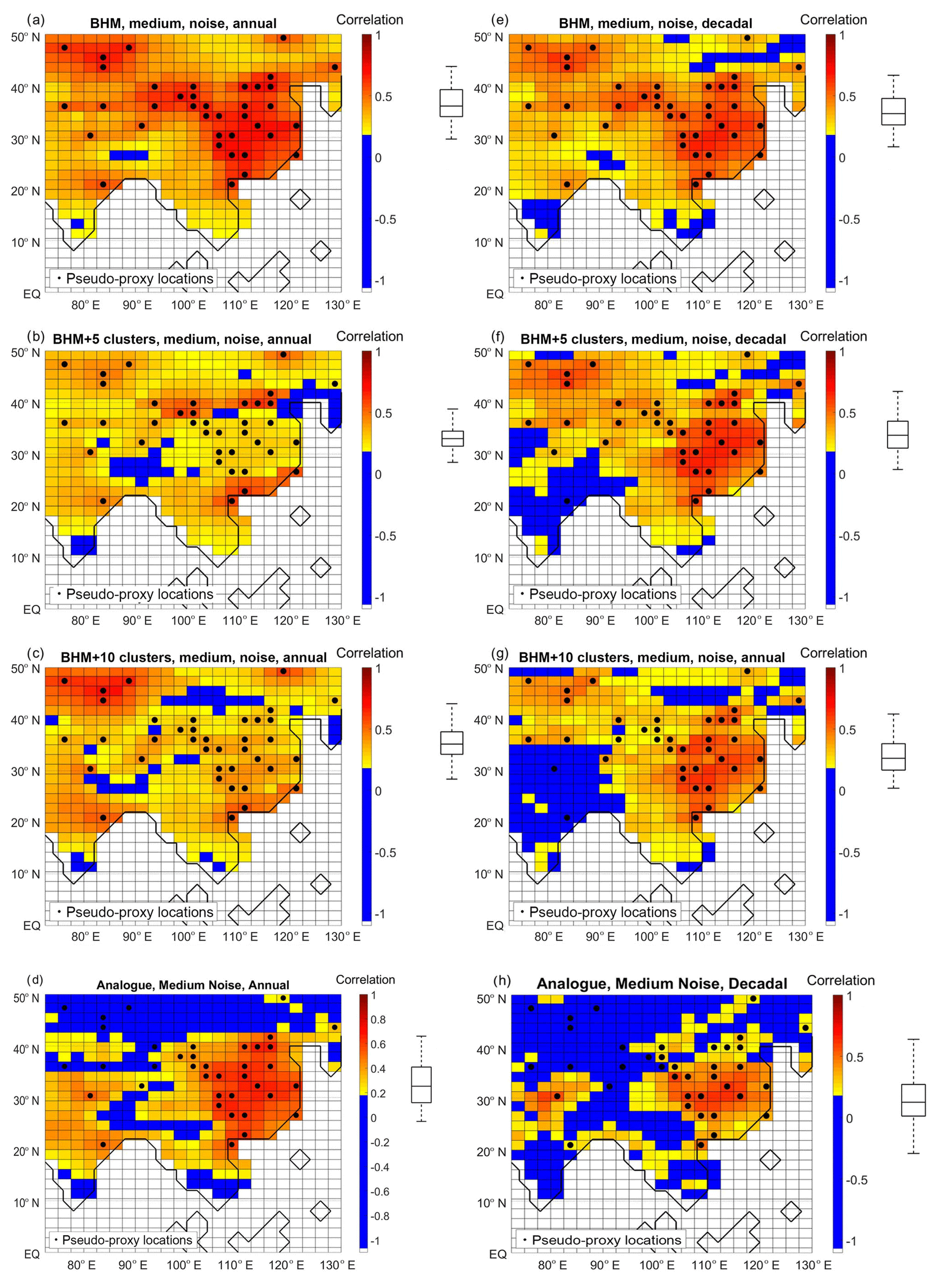
Figure 4Correlation between target precipitation and different reconstructions, at each grid point. (a, b, c, d) Annually resolved data. (e, f, g, h) Decadally resolved data. (a, e) BHM. (b, f) BHM+5Clusters. (c, g) BHM+10Clsuters. (d, h) Analogue method. The boxplots (indicating median, 25 %, and 75 % percentiles and non-outlier limits) to the right of the colour bars show the distribution of the grid-point correlation coefficients. Black dots: pseudo-proxy network.
For the annual-resolution reconstructions, the best performance is obtained by the BHM technique, showing a spatial mean correlation with the target of 0.4 (Fig. 4a). Coupling the BHM with clustering partially deteriorates the results, with the correlation coefficient severely dropping over the proxy-rich EChina region (Fig. 4b and c). Meanwhile, the performance of the analogue method is inferior: the correlation coefficient spatial mean is 0.25 and there is no skill in reconstructing precipitation north of 42∘ N despite the fact that pseudo-proxies are located in that region (Fig. 4d).
For the decadally resolved reconstructions the difference between the Bayesian methods and the analogue is even larger. In terms of the correlation coefficient measure the BHM (analogue method) is the best (worst) performing, with a spatial average of 0.37 (0.1). Among the Bayesian schemes, the cluster coupling maintains the skill levels in all regions except India, where lower correlation values are obtained. The analogue method shows a much constrained geographical skill, with correlation values above 0.2 only over EChina and central India.
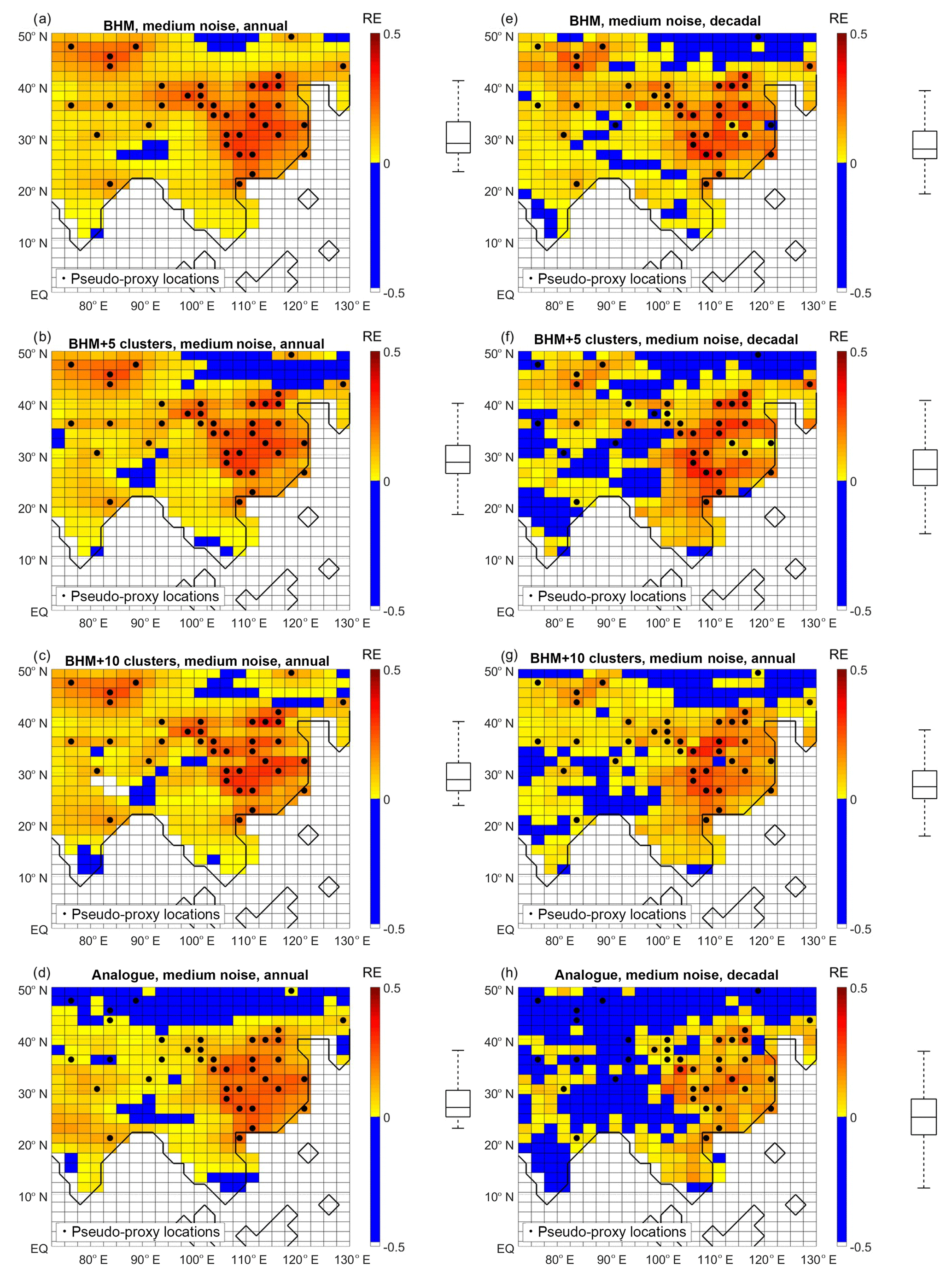
Figure 5RE index for different reconstructions, at each grid point. (a, b, c, d) Annually resolved data. (e, f, g, h) Decadally resolved data. (a, e) BHM. (b, f) BHM+5Clusters. (c, g) BHM+10Clsuters. (d, h) Analogue method. The boxplots (indicating median, 25 % and 75 % percentiles and non-outlier limits) to the right of the colour bars show the distribution of the grid-point RE index. Black dots: pseudo-proxy network.
In general, for each of the methods, the correlation coefficient is higher for the annually resolved than for the decadally resolved reconstruction. One exception to that is the BHM+5Clusters over EChina. This behaviour is probably derived from the clustering division (see Fig. A2).
Figure 5 shows the results for the RE index. In most of the grid points the RE index is positive, indicating a reduction of the error in comparison to forecasting the instrumental-period climatology as a reconstruction. For all the Bayesian methods and both time resolutions the highest skill is found in regions with high density of pseudo-proxy information. Again, the analogue method shows a clearly inferior performance to NWAChina, in spite of the considerable number of pseudo-proxy locations present there.
For the annual reconstruction, improvements from climatology are found for the Bayesian approaches in EChina, NWAChina, Mongolia and, to a lesser extent, in central India (Fig. 5a, b and c). For the analogue method, the improvement with respect to climatology is confined only to EChina and central India, and the improvement is weaker than with the Bayesian techniques (Fig. 5d).
For the decadal data, similar results are obtained. However, the RE index is notably negative in some grid points for the BHM+5clusters (mainly in the northern-most extent of the study region; Fig. 5f) and the analogue cases (everywhere with the exception of EChina; Fig. 5h).
Figure 6 displays the results for the CRPS metric, for the probabilistic methods (Bayesian schemes). For this metric, the annually resolved (decadally resolved) reconstructions have a CRPS of 190 mm per month (22 mm per month), compared to the target precipitation spatially averaged standard deviation of 34 mm per month (11 mm per month) for annual (decadal) data. This indicates that the methods have more problems in reproducing the expected probability distribution functions in the annual case.
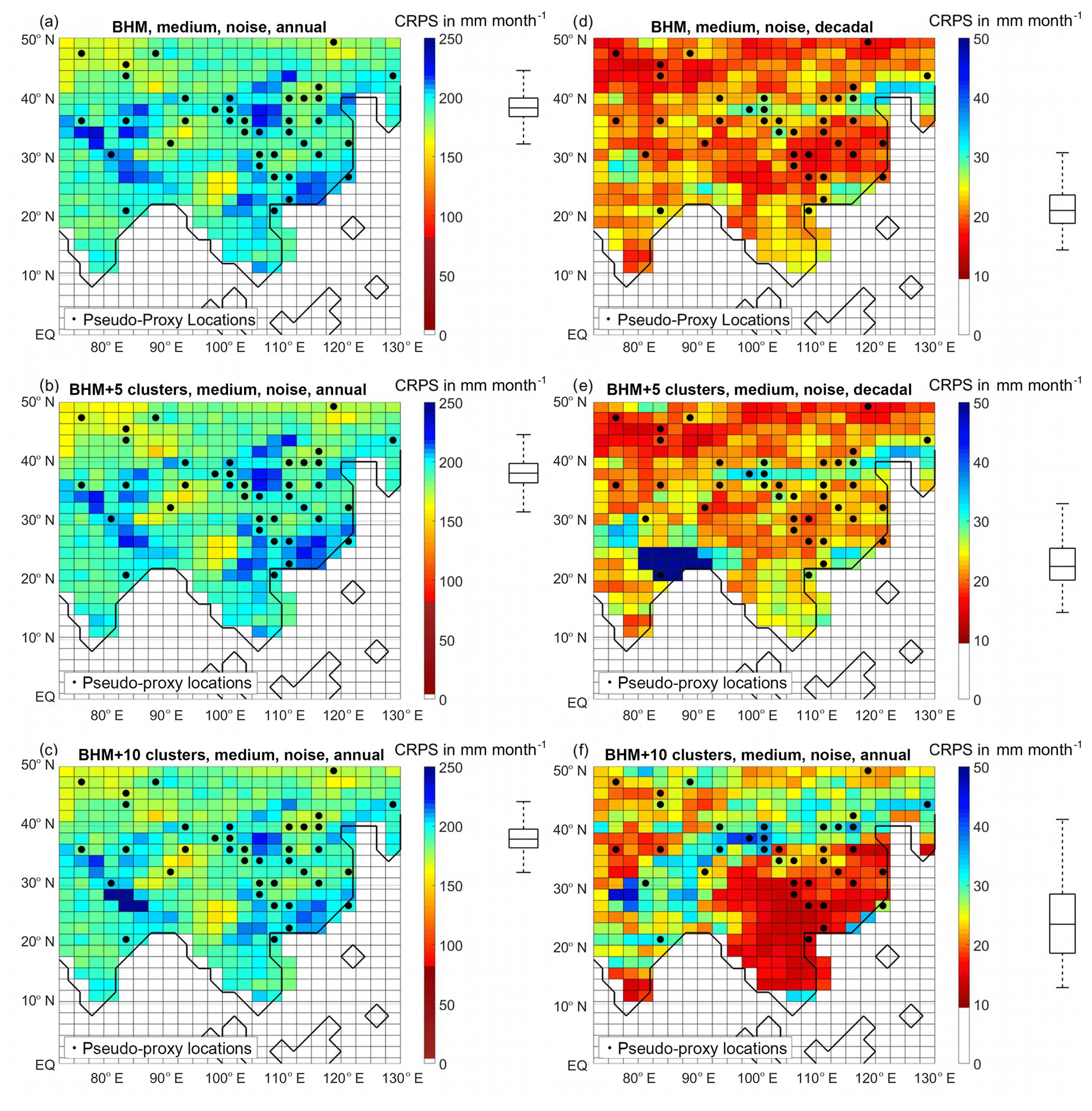
Figure 6CRPS for different reconstructions, at each grid point. (a, b, c) Annually resolved data. (d, e, f) Decadally resolved data. (a, d) BHM reconstruction. (b, e) BHM+5Clusters. (c, f) BHM+10Clusters. The boxplots (indicating median, 25 % and 75 % percentiles and non-outlier limits) to the right of the colour bars show the distribution of the grid-point CRPS. Black dots: pseudo-proxy network.
For the annual-resolution reconstructions there is almost no noticeable difference in the performance of the three Bayesian schemes. For this metric, the region of best performance is NWAChina. In this case, the performance over the proxy-rich EChina is intermediate (unlike with the correlation coefficient and RE index metrics). For the decadal-resolution reconstructions, the performance among the methods is quite different. While the spatial mean is in all three cases similar (around 22 mm per month), the spread among grid points is much higher for the BHM+10Clusters scheme. In particular, for the 10-cluster scheme the skill over China and the south-east of the study region is much higher than in the other methods. In general, the regions with a dense proxy network display better performance levels, and central India and the north-east of the study area stand out as low-performing areas for all three methodologies.
Three main conclusions can be drawn from the experiments above: first, proxy-depleted areas cannot be successfully reconstructed. Second, the Bayesian schemes are superior to the analogue method in all metrics (this difference is particularly acute over NWAChina, where the analogue method fails despite the relatively good coverage by proxy data). Third, among the Bayesian algorithms the results are similar, although a partial deterioration of the skill is detected in some regions when clustering is coupled.
The underperformance of the analogue method in comparison with the BHM variants might seem in contradiction with the results of Gómez-Navarro et al. (2015), who do not find any significant skill differences between these schemes. However, we should note an important difference between the two studies: in Gómez-Navarro et al. (2015) the authors use as their pool of analogues an independent highly resolved simulation performed with a regional model, while in this paper we use the classical analogue approach based on the instrumental-period pool. This difference makes it impossible to draw a fair comparison between the two studies, indicating that the pool of analogues is essential for determining the potential success of the analogue method as a reconstruction technique.
We hypothesise a couple of reasons for the failure of the analogue method over NWAChina: first, the semi-arid precipitation regime dominant in the area and, second, an insufficient number of analogues in the pool. As the method is unsuccessful at both annual and decadal resolutions, we think that the number of elements in the pool of analogues is not an important variable and that the main cause of the failure resides in the fact that non-normal-behaving time series could potentially be more difficult to mimic by analogues than Gaussian-behaving ones. However, providing a proof of such a hypothesis is out of the scope of this paper and will require the design of new theoretical experiments with input data arising from different probability distributions.
Disentangling the reasons leading to a partial deterioration of skill when coupling the BHM to clustering algorithms will require additional experiments. However, we hypothesise that the main reason for such behaviour is related to the loss of information from geographical neighbours. While during clustering geographical neighbours can be separated, the information from such sites is taken into account in the covariance matrix structure of BHM and, therefore, losing information from close locations might affect the final performance.
3.2 Effect of noise in pseudo-proxy records
Next, we evaluate the impact of noise in the pseudo-proxy time series on the skill of the reconstruction techniques. We focus on two schemes: one Bayesian (BHM+5Clusters, selected for its balance between skill and computational requirements, as shown in Sect. 3.1) and the analogue method. We work with four noise levels for the pseudo-proxy time series: high noise (correlation with truth: 0.3), medium noise (correlation with truth: 0.5), low noise (correlation with truth: 0.7) and perfect proxy (correlation with truth: 1). Note that the medium-noise proxy case corresponds to the level used through Sect. 3.1. To simplify and summarise the results, in this subsection we display the reconstruction performance in terms of only one skill measure: the correlation coefficient.
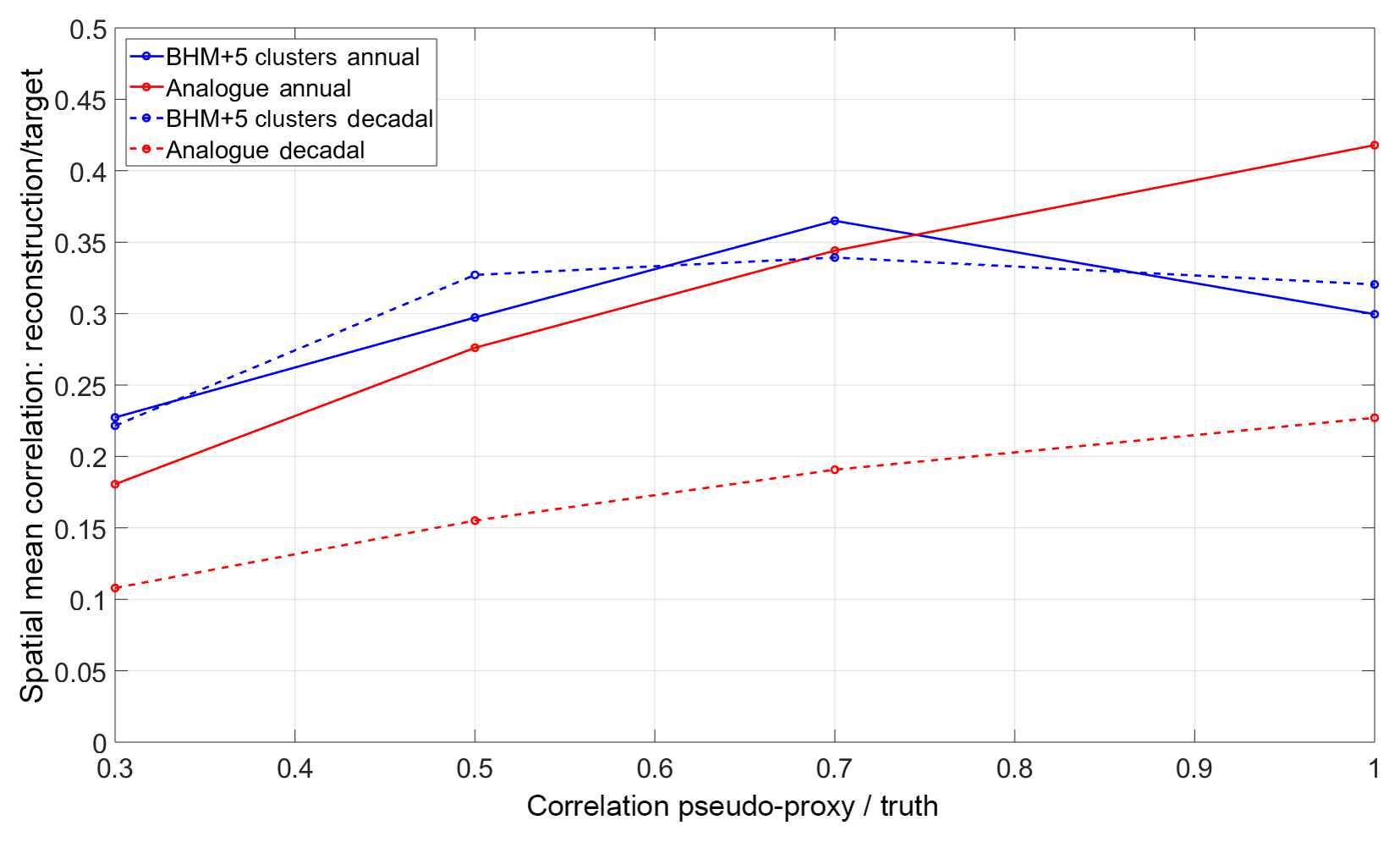
Figure 7Spatial mean correlation skill of reconstruction techniques for different noise levels (expressed here in terms of the correlation between the pseudo-proxy and truth).
Figure 7 shows the dependency of the correlation coefficient, averaged in space, with noise levels in the pseudo-proxy records. At annual resolution, the skill of the methods increases in an almost linear way with the quality of the pseudo-proxy records, except for a drop in the Bayesian skill in the no-noise scenario. The BHM+5Clusters performance is better than the analogue method in all cases except the no-noise one. For high-noise proxies the skill of the BHM+5Clusters (analogue method) is 0.23 (0.18), while in the perfect-proxy scenario the BHM+5Clusters (analogue method) reaches 0.30 (0.42). For decadally resolved reconstructions the picture is quite different. The Bayesian approaches show a quasi-constant skill for the medium, low and no-noise examples (around 0.33) and the analogue method performs poorly, showing for all the noise types a skill between 0.09 and 0.15. While for the Bayesian schemes the spatial average skill for the annual or decadal resolutions is similar, the difference between annual versus decadal is important in the analogue case. To complement the spatially averaged information, Figs. 8 and 9 show the sensitivity of the correlation skill measure field to the noise levels in the pseudo-proxies for the BHM+5Clusters and the analogue method, respectively.

Figure 8BHM+5Clusters performance in terms of correlation with the target for different levels of noise at annual (a, b, c, d) or decadal (e, f, g, h) resolution. (a, b) No noise. (c, d) Low noise. (e, f) Medium-level noise. (g, h) High noise. The boxplots (indicating median, 25 % and 75 % percentiles and non-outlier limits) to the right of the colour bars show the distribution of the grid-point correlation coefficients. Black dots: pseudo-proxy network.
For the Bayesian algorithm (Fig. 8), the perfect-proxy case shows high performance over NWAChina, EChina and north-east of the study area, at annual and decadal resolutions. For the annual reconstruction, the skill of the scheme is low southward of 25∘ N and over some grid cells in the north of the area. For the decadal reconstruction, the same areas are also problematic and, in addition, most of India is not well reconstructed. In general, as the noise level in the input pseudo-proxies increases, the performance of the method deteriorates, and for the high-noise case only East China and the north-west of the study region show moderate success.
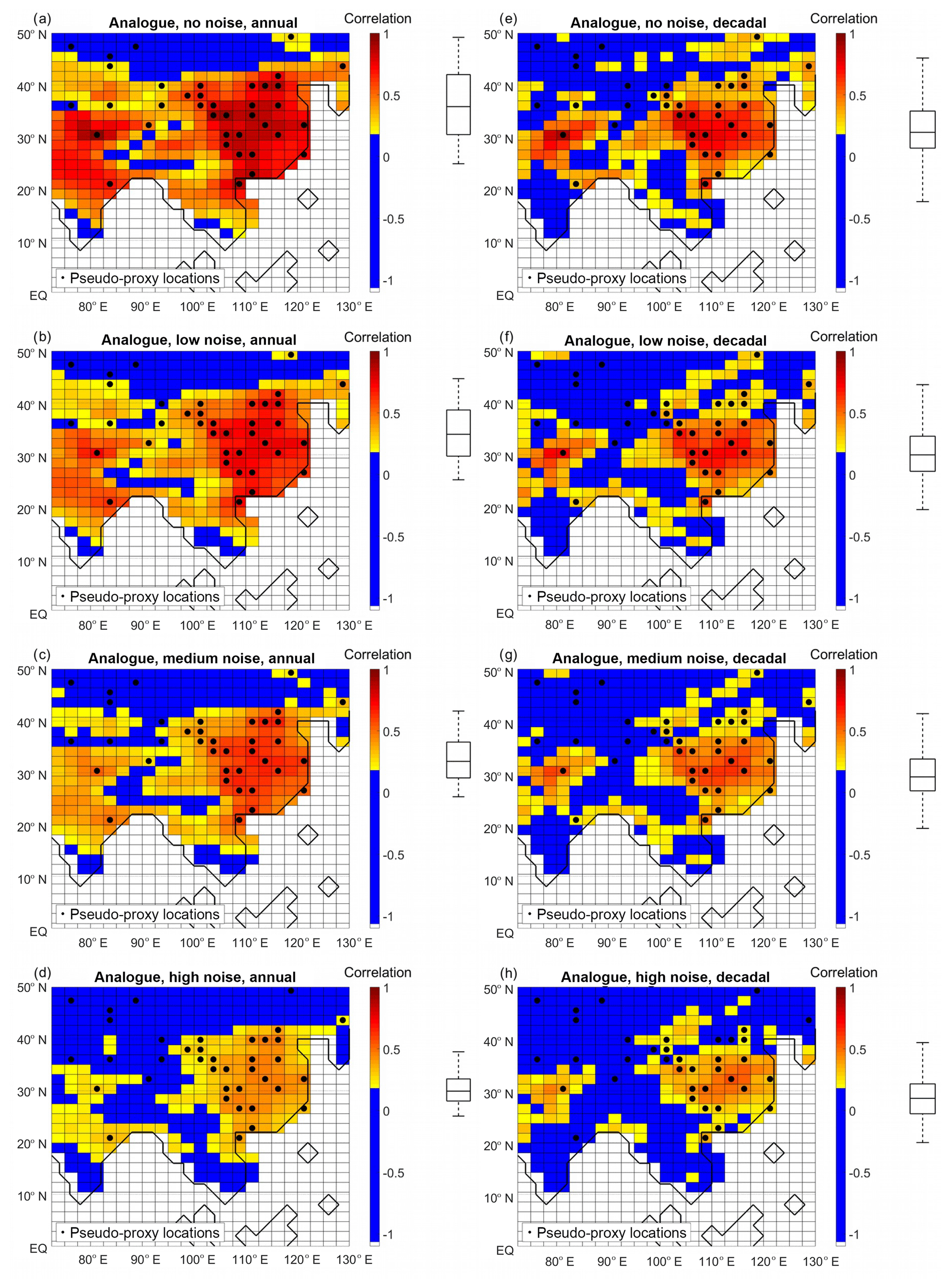
Figure 9Analogue method performance in terms of correlation with target for different levels of noise at annual (a, b, c, d) or decadal (e, f, g, h) resolution. (a, b) No noise. (c, d) Low noise. (e, f) Medium-level noise. (g, h) High noise. The boxplots (indicating median, 25 % and 75 % percentiles and non-outlier limits) to the right of the colour bars show the distribution of the grid-point correlation coefficients. Black dots: pseudo-proxy network.
Figure 9 presents the analogue method performance. For annual resolution, in the case of perfect pseudo-proxies, the method is successful in the central part of the study area (between 15 and 45∘ N), while the northern and southern-most extremes are not well reconstructed. However, the decadal counterpart is only skilful in EChina. At the high-noise end of the spectrum, the analogue method only shows a satisfactory performance in EChina, between 20 and 40∘ N (between 25 and 35∘ N) for the annually resolved (decadally resolved) reconstruction.
To summarise, as expected, the noise in the pseudo-proxy time series is important, as the quality of the reconstruction rapidly decreases with the noise level.
This study evaluates the ability of several statistical techniques to reconstruct the precipitation field over south-eastern Asia in a PPE setting. The reconstructions are performed using 1156 years of model simulation (corresponding to the period 850–2005), at annual and decadal resolution. The techniques used are BHM, BHM coupled with clustering (dividing south-eastern Asia into 5 or 10 clusters) and the analogue method. While the analogue method is a classical approach and has been widely used, the Bayesian variants are novel for the hydro-climatological reconstructions' field, this being the first time the technique is applied for Asian precipitation reconstruction. Moreover, the coupling of the Bayesian modelling with clustering algorithms is also an innovation that could potentially lead to a more widespread application of these computationally intensive processes.
We find that for all the algorithms and resolutions a high density of pseudo-proxy information is a necessary but not sufficient condition for a successful reconstruction. On the one hand, the lack of proxy data over regions such as the north-east of the study area, south of Tibet and south of 20∘ N, determines that none of the methods is capable of delivering a skilful reconstruction. On the other hand, a good performance over the proxy-rich areas of EChina and NWAChina is not guaranteed just by the amount of data present there: while all the methods are highly successful over EChina, only the Bayesian algorithms deliver quality reconstructions over NWAChina.
Among the three Bayesian schemes the differences in skill are not extremely notorious, although a partial deterioration of the skill is detected in some regions when clustering is coupled. Noting that the Bayesian technique without any form of pre-clustering of the area of interest (BHM) is extremely computationally expensive, coupling it with a clustering scheme (BHM+5Clusters or BHM+10Clusters) seems to be a good compromise between success of the reconstruction and computational demand (with computing times reduced by up to 50 %).
We also find that the quality of the final reconstructions is highly sensitive to the noise levels included in the input pseudo-proxy data, those variables being negatively correlated. Only under a perfect-proxy (no-noise) scenario and at annual resolution is the analogue method capable of overperforming the Bayesian schemes over most areas. Even in this ideal no-noise case NWAChina remains elusive for the analogue methodology.
As a summary, we find that for millennium-length precipitation reconstructions over south-eastern Asia a dense network of proxy information is mandatory for success, highlighting the complex nature of the precipitation field in the area of study. Among the selected algorithms, the Bayesian techniques perform generally better than the analogue method, the difference in abilities being highest over the semi-arid north-west and in the decadal-resolution framework. The superiority of the Bayesian approach indicates that directly modelling the space and time precipitation field variability is more appropriate than just relying on similarities within a restricted pool of observational analogues, in which certain regimes might not be present.
A natural next step is to implement real-world reconstructions of precipitation in the region of continental south-eastern Asia. These PPEs are auspicious for such a future endeavour, as some moderate skill can be expected in most of the region. Nevertheless, it is important to acknowledge that these experiments are highly idealised and that real-world data might incorporate additional constraints and challenges. Additionally, more PPEs could also be designed by omitting some of the simplifications assumed here. For example, while here we only took proxy time series that cover the whole period of interest, with the same temporal resolution, same signal to noise relation and same relationship with the underlying hydroclimatic variable of interest, some of these constraints could be modified to better resemble reality.
Data sets, codes and analysis scripts used in this study can be obtained from: https://doi.org/10.17605/OSF.IO/B2RXP (Talento, 2019).

Figure A1Kolmogorov–Smirnov normality test on the simulated JJA precipitation during the instrumental period (years 1906–2005, at annual resolution). (a) Rejection or acceptance of the normality hypothesis, at a 95 % confidence level; (b) p values. Black dots: pseudo-proxy network.
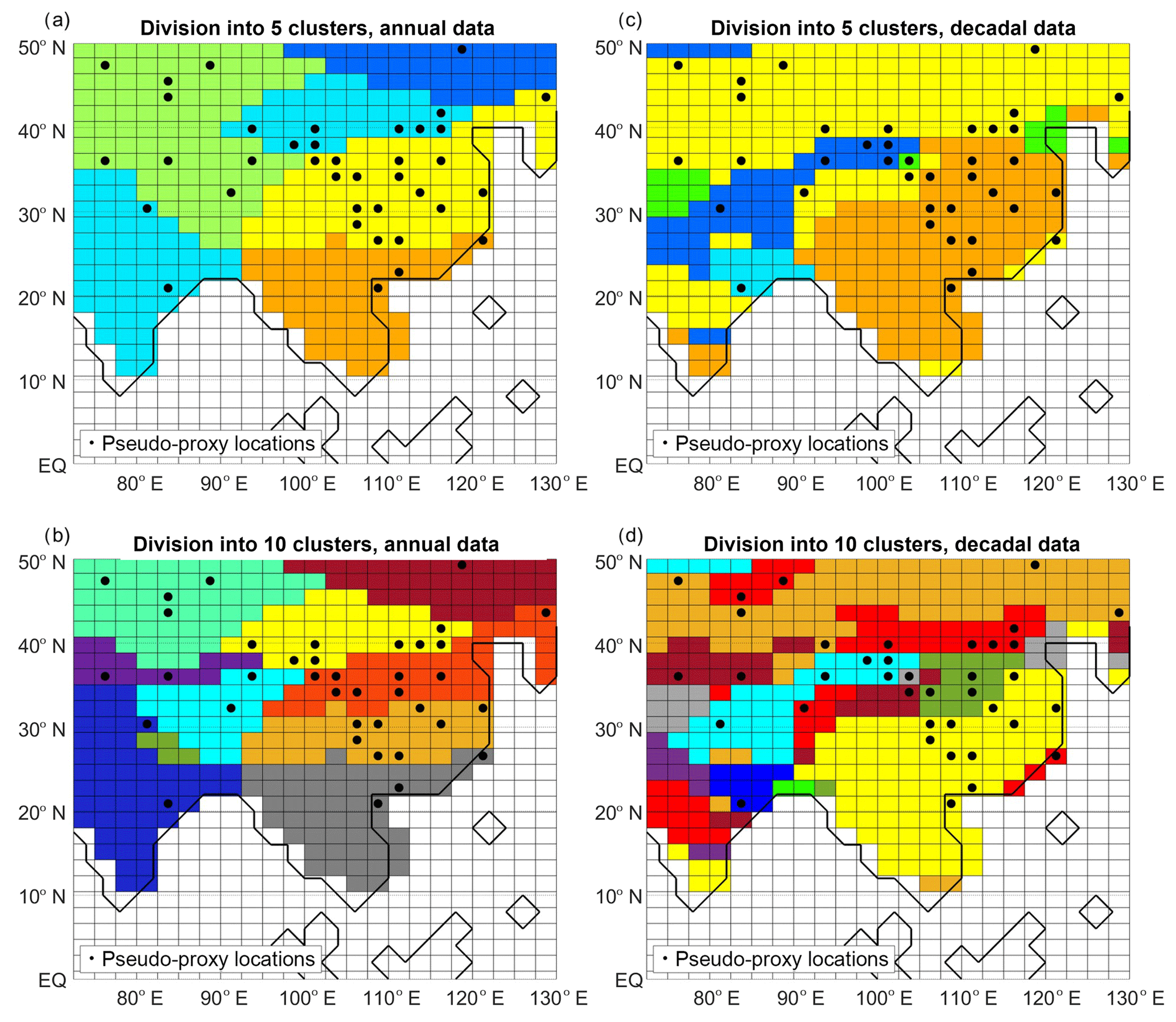
Figure A2Divisions into clusters (in each plot different colors indicate different clusters), using the simulated JJA precipitation in the instrumental period (years 1996–2005) as input. (a) Annual data, division into 5 clusters, (b) annual data, division into 10 clusters, (c) decadal data, division into 5 clusters, and (d) decadal data, division into 10 clusters. Magenta dots: pseudo-proxy network.
ST made all the calculations, produced all the figures and wrote the main text. LS, JW and JL contributed with discussions and comments on the manuscript.
The authors declare that they have no conflict of interest.
This article is part of the special issue “Hydro-climate dynamics, analytics and predictability”. It is not associated with a conference.
Stefanie Talento, Lea Schneider and Jürg Luterbacher are supported by the Belmont Forum and JPI-Climate Collaborative Research Action “INTEGRATE: An integrated data-model study of interactions between tropical monsoons and extratropical climate variability and extremes”. Jürg Luterbacher acknowledges support by the UK–China Research and Innovation Partnership Fund through the Met Office Climate Science for Service Partnership China (CSSP) as part of the Newton Fund.
The authors thank the reviewers for constructive criticism and suggestions that improved the quality of the paper. The authors also thank the proxy and model data providers.
This research has been supported by the Belmont Forum, JPI-Climate
(INTEGRATE grant).
This open-access publication was funded
by Justus Liebig
University.
This paper was edited by Naresh Devineni and reviewed by Tine Nilsen and one anonymous referee.
Cai, Y., Tan, L., Cheng, H., An, Z., Edwards, R. L., Kelly, M. J., Kong, X., and Wang, X.: The variation of summer monsoon precipitation in central China since the last deglaciation, Earth Planet. Sc. Lett., 291, 21–31, https://doi.org/10.1016/j.epsl.2009.12.039, 2010.
Chen, J., Chen, F., Feng, S., Huang, W., Liu, J., and Zhou, A.: Hydroclimatic changes in China and surroundings during the Medieval Climate Anomaly and Little Ice Age: spatial patterns and possible mechanisms, Quaternary Sci. Rev., 107, 98–111, https://doi.org/10.1016/j.quascirev.2014.10.012, 2015.
Chu, G., Sun, Q., Wang, X., Li, D., Rioual, P., Qiang, L., Han, J., and Liu, J.: A 1600 year multiproxy record of paleoclimatic change from varved sediments in Lake Xiaolongwan, northeastern China, J. Geophys. Res., 114, D22108, https://doi.org/10.1029/2009JD012077, 2009.
Cook, E. R., Briffa, K. R., and Jones, P. D.: Spatial regression methods in dendroclimatology: a review and comparison of two techniques, Int. J. Climatol., 14, 379–402, https://doi.org/10.1002/joc.3370140404, 1994.
Cook, E. R., Anchukaitis, K. J., Buckley, B. M., D'Arrigo, R. D., Jacoby, G. C., and Wright, W. E. X.: Asian monsoon failure and megadrought during the last millennium, Science, 328, 486–489, 2010.
Feng, S., Hu, Q., Wu, Q., and Mann, M. E.: A gridded reconstruction of warm season precipitation for Asia spanning the past half millennium, J. Climate, 26, 2192–2204, https://doi.org/10.1175/JCLI-D-12-00099.1, 2013.
Feng, Z.-D., Wu, H. N., Zhang, C. J., Ran, M., and Sun, A. Z.: Bioclimatic change of the past 2500 years within the Balkhash Basin, eastern Kazakhstan, Central Asia, Quatern. Int., 311, 63–70, https://doi.org/10.1016/j.quaint.2013.06.032, 2013.
Franke, J., González-Rouco, J. F., Frank, D., and Graham, N. E.: 200 years of European temperature variability: insights from and tests of the proxy surrogate reconstruction analog method, Clim. Dynam., 37, 133–150, https://doi.org/10.1007/s00382-010-0802-6, 2011.
Gelman, A., Carlin, J., Stern, H., and Rubin, D.: Bayesian Data Anal, 3rd edn., Chapman and Hall, London, 2003.
Gómez-Navarro, J. J., Werner, J., Wagner, S., Luterbacher, J., and Zorita, E.: Establishing the skill of climate field reconstruction techniques for precipitation with pseudoproxy experiments, Clim. Dynam., 45, 1395–1413, https://doi.org/10.1007/s00382-014-2388-x, 2015.
Gong, G. and Hameed, S.: The variation of moisture conditions in China during the last 2000 years, Int. J. Climatol., 11, 271–283, https://doi.org/10.1002/joc.3370110304, 1991.
Gou, X., Deng, Y., Chen, F., Yang, M., Fang, K., Gao, L., Yang, T., and Zhang, F.: Tree ring based streamflow reconstruction for the Upper Yellow River over the past 1234 years, Chinese Sci. Bull., 55, 4179–418, https://doi.org/10.1007/s11434-010-4215-z, 2010.
Guillot, D., Rajaratnam, B., and Emile-Geay, J.: Statistical paleoclimate reconstructions via Markov random fields, Ann. Appl. Stat., 9, 324–352, https://doi.org/10.1214/14-AOAS794, 2015.
He, M., Bräuning, A., Grießinger, J., Hochreuther, P., and Wernicke, J.: May–June drought reconstruction over the past 821 years on the south-central Tibetan Plateau derived from tree-ring width series, Dendrochronologia, 47, 48–57, https://doi.org/10.1016/j.dendro.2017.12.006, 2018.
He, Y., Zhao, C., Wang, Z., Wang, H., Song, M., Liu, W., and Liu, Z.: Late Holocene coupled moisture and temperature changes on the northern Tibetan Plateau, Quaternary Sci. Rev., 80, 47–57, https://doi.org/10.1016/j.quascirev.2013.08.017, 2013.
Hersbach, H.: Decomposition of the continuous ranked probability score for ensemble prediction systems, Weather Forecast., 15, 559–570, https://doi.org/10.1175/1520-0434(2000)015<0559:DOTCRP>2.0.CO;2, 2000.
Hong, Y. T., Hong, B., Lin, Q. H., Shibata, Y., Hirota, M., Zhu, Y. X., Leng, X. T., Wang, Y., Wang, H., and Yi, L.: Inverse phase oscillations between the East Asian and Indian Ocean summer monsoons during the last 12000 years and paleo-El Niño, Earth Planet. Sc. Lett., 231, 337–346, https://doi.org/10.1016/j.epsl.2004.12.025, 2005.
Hu, C., Henderson, G. M., Huang, J., Xie, S., Sun, Y., and Johnson, K. R.: Quantification of Holocene Asian monsoon rainfall from spatially separated cave records, Earth Planet. Sc. Lett., 266, 221–232, https://doi.org/10.1016/j.epsl.2007.10.015, 2008.
Izenman, A. J.: Modern Multivariate Statistical Techniques, Springer Texts in Statistics, Springer-Verlag New York, 2008.
Jiang, T., Zhang, Q., Blender, R., and Fraedrich, K.: Yangtze Delta floods and droughts of the last millennium: Abrupt changes and long term memory, Theor. Appl. Climatol., 82, 131–141, https://doi.org/10.1007/s00704-005-0125-4, 2005
Jones, P. D., Briffa, K. R., Osborn, T. J., Lough, J. M., van Ommen, T. D., Vinther, B. M., Luterbacher, J., Wahl, E., Zwiers, F. W., Schmidt, G. A., Ammann, C., Mann, M. E., Buckley, B. M., Cobb, K., Esper, J., Goosse, H., Graham, N., Jansen, E., Kiefer, T., Kull, C., Küttel, M., Mosley-Thompson, E., Overpeck, J. T., Riedwyl, N., Schulz, M., Tudhope, S., Villalba, R., Wanner, H., Wolff, E., and Xoplaki, E.: High-resolution palaeoclimatology of the last millennium: a review of current status and future prospects, Holocene, 19, 3–49, https://doi.org/10.1177/0959683608098952, 2009.
Kasper, T., Haberzettl, T., Doberschütz, S., Daut, G., Wang, J., Zhu, L., Nowaczyk, N., and Mäusbacher, R.: Indian Ocean Summer Monsoon (IOSM)-dynamics within the past 4 ka recorded in the sediments of Lake Nam Co, central Tibetan Plateau (China), Quaternary Sci. Rev., 39, 73–85, https://doi.org/10.1016/j.quascirev.2012.02.011, 2012.
Kuo, T. S., Liu, Z. Q., Li, H. C., Wan, N. J., Shen, C. C., and Ku, T. L.: Climate and environmental changes during the past millennium in central western Guizhou, China as recorded by Stalagmite ZJD-21, J. Asian Earth Sci., 40, 1111–1120, https://doi.org/10.1016/j.jseaes.2011.01.001, 2011.
Li, H. C., Lee, Z. H., Wan, N. J., Shen, C. C., Li, T. Y., Yuan, D. X., and Chen, Y. H.: The δ18O and δ13C records in an aragonite stalagmite from Furong Cave, Chongqing, China: A-2000-year record of monsoonal climate, J. Asian Earth Sci., 40, 1121–1130, https://doi.org/10.1016/j.jseaes.2010.06.011, 2011.
Liangcheng, T., Yanjun, C., Liang, Y., Zhisheng, A., and Li, A.: Precipitation variations of Longxi, northeast margin of Tibetan Plateau since AD 960 and their relationship with solar activity, Clim. Past, 4, 19–28, https://doi.org/10.5194/cp-4-19-2008, 2008.
Liu, J., Chen, F., Chen, J., Xia, D., Xu, Q., Wang, Z., and Li, Y.: Humid medieval warm period recorded by magnetic characteristics of sediments from Gonghai Lake, Shanxi, North China, Chinese Sci. Bull., 56, 2464–2474, https://doi.org/10.1007/s11434-011-4592-y, 2011.
Liu, X., Herzschuh, U., Shen, J., Jiang, Q., and Xiao, X.: Holocene environmental and climatic changes inferred from Wulungu Lake in northern Xinjiang, China, Quaternary Res., 70, 412–425, https://doi.org/10.1016/j.yqres.2008.06.005, 2008.
Liu, X., Dong, H., Yang, X., Herzschuh, U., Zhang, E., Stuut, J.-B. W., and Wang, Y.: Late Holocene forcing of the Asian winter and summer monsoon as evidenced by proxy records from the northern Qinghai–Tibetan Plateau, Earth Planet. Sc. Lett., 280, 276–284, https://doi.org/10.1016/j.epsl.2009.01.041, 2009.
Liu, Z., Liu, Q., Torrent, J., Barrón, V., and Hu, P.: Testing the magnetic proxy χFD/HIRM for quantifying paleoprecipitation in modern soil profiles from Shaanxi Province, China, Global Planet. Change, 110, 368–378, https://doi.org/10.1016/j.gloplacha.2013.04.013, 2013.
Ljungqvist, F. C., Krusic, P. J., Sundqvist, H. S., Zorita, E., Brattström, G., and Frank, D.: Northern Hemisphere hydroclimate variability over the past twelve centuries, Nature, 532, 94–98, https://doi.org/10.1038/nature17418, 2016.
Lorenz, E. N.: Atmospheric predictability as revealed by naturally occurring analogues, J. Atmos. Sci., 26, 636–646, 1969.
Luterbacher, J. and Zorita, E.: Spatial climate field reconstructions, in: The Palgrave Handbook of Climate History, edited by: White, S., Pfister, C., and Mauelshagen, F., Palgrave Macmillan, UK, 131–139, 2018.
Luterbacher, J., Werner, J. P., Smerdon, J. E., et al.: European summer temperatures since Roman times, Environ. Res. Lett., 11, 024001, https://doi.org/10.1088/1748-9326/11/2/024001, 2016.
Mann, M. E. and Rutherford, S.: Climate reconstruction using “Pseudoproxies”, Geophys. Res. Lett., 29, 139-1–139-4, https://doi.org/10.1029/2001GL014554, 2002.
Nilsen, T., Werner, J. P., Divine, D. V., and Rypdal, M.: Assessing the performance of the BARCAST climate field reconstruction technique for a climate with long-range memory, Clim. Past, 14, 947–967, https://doi.org/10.5194/cp-14-947-2018, 2018.
Otto-Bliesner, B. L., Brady, E. C., Fasullo, J., Jahn, A., Landrum, L., Stevenson, S., Rosenbloom, N., Mai, A., and Strand, G.: Climate variability and change since 850 CE: An ensemble approach with the Community Earth System Model, B. Am. Meteorol. Soc., 97, 735–754, https://doi.org/10.1175/BAMS-D-14-00233.1, 2016.
Paulsen, D. E., Li, H. C., and Ku, T. L.: Climate variability in central China over the last 1270 years revealed by high-resolution stalagmite records, Quaternary Sci. Rev., 22, 691–701, https://doi.org/10.1016/S0277-3791(02)00240-8, 2003.
Qian, W., Hu, Q., Zhu, Y., and Lee, D. K.: Centennial-scale dry-wet variations in East Asia, Clim. Dynam., 21, 77–89, https://doi.org/10.1007/s00382-003-0319-3, 2003.
Sanwal, J., Kotlia, B. S., Rajendran, C., Ahmad, S. M., Rajendran, K., and Sandiford, M.: Climatic variability in Central Indian Himalaya during the last ∼1800 years: Evidence from a high resolution speleothem record, Quaternary Int., 304, 183–192, https://doi.org/10.1016/j.quaint.2013.03.029, 2013.
Schneider, T.: Analysis of incomplete climate data: Estimation of mean values and covariance matrices and imputation of missing values, J. Climate, 14, 853–871, https://doi.org/10.1175/1520-0442(2001)014<0853:AOICDE>2.0.CO;2, 2001.
Sheppard, P. R., Tarasov, P. E., Graumlich, L. J., Heussner, K. U., Wagner, M., Sterle, H., and Thompson, L. G.: Annual precipitation since 515 BC reconstructed from living and fossil juniper growth of northeastern Qinghai Province, China, Clim. Dynam., 23, 869–881, https://doi.org/10.1007/s00382-004-0473-2, 2004.
Shi, F., Li, J., and Wilson, R. J.: A tree-ring reconstruction of the South Asian summer monsoon index over the past millennium, Scientific Reports, 4, 6739, https://doi.org/10.1038/srep06739, 2014.
Shi, F., Zhao, S., Guo, Z., Goosse, H., and Yin, Q.: Multi-proxy reconstructions of May–September precipitation field in China over the past 500 years, Clim. Past, 13, 1919–1938, https://doi.org/10.5194/cp-13-1919-2017, 2017.
Sinha, A., Berkelhammer, M., Stott, L., Mudelsee, M., Cheng, H., and Biswas, J.: The leading mode of Indian Summer Monsoon precipitation variability during the last millennium, Geophys. Res. Lett., 38, L15703, https://doi.org/10.1029/2011GL047713, 2011.
Smerdon, J. E.: Climate models as a test bed for climate reconstruction methods: pseudoproxy experiments, WIREs Clim. Change, 3, 63–77, https://doi.org/10.1002/wcc.149, 2012.
Smerdon, J. E., Kaplan, A., Chang, D., and Evans, M. N.: A pseudoproxy evaluation of the CCA and RegEM methods for reconstructing climate fields of the last millennium, J. Climate, 23, 4856–4880, 2010.
Sun, A. and Feng, Z.: Holocene climatic reconstructions from the fossil pollen record at Qigai Nuur in the southern Mongolian Plateau, Holocene, 23, 1391–1402, https://doi.org/10.1177/0959683613489581, 2013.
Talento, S.: Data: Millennium-length precipitation Reconstruction over South-eastern Asia: a Pseudo-Proxy Approach, https://doi.org/10.17605/OSF.IO/B2RXP, 2019.
Tan, L., Cai, Y., An, Z., Edwards, R. L., Cheng, H., Shen, C. C., and Zhang, H.: Centennial- to decadal-scale monsoon precipitation variability in the semi-humid region, northern China during the last 1860 years: Records from stalagmites in Huangye Cave, Holocene, 21, 287–296, https://doi.org/10.1177/0959683610378880, 2011.
Tingley, M. P. and Huybers, P.: A Bayesian algorithm for reconstructing climate anomalies in space and time. Part I: Development and applications to paleoclimate reconstruction problems, J. Climate, 23, 2759–2781, https://doi.org/10.1175/2009JCLI3015.1, 2010.
Tingley, M. P. and Huybers, P.: Recent temperature extremes at high northern latitudes unprecedented in the past 600 years, Nature, 496, 201–205, https://doi.org/10.1038/nature11969, 2013.
Treydte, K. S., Schleser, G. H., Helle, G., Frank, D. C., Winiger, M., Haug, G. H., and Esper, J.: The twentieth century was the wettest period in northern Pakistan over the past millennium, Nature, 440, 1179–1182, https://doi.org/10.1038/nature04743, 2006.
Wang, Z., Li, Y., Liu, B., and Liu, J.: Global climate internal variability in a 2000-year control simulation with Community Earth System Model (CESM), Chinese Geogr. Sci., 25, 263–273, https://doi.org/10.1007/s11769-015-0754-1, 2015.
Wang, Y., Cheng, H., Edwards, R. L., He, Y., Kong, X., An, Z. S., Wu, J., Kelly, M. J., Dykoski, C. A., and Li, X.: The Holocene Asian Monsoon: Links to Solar Changes and North Atlantic Climate, Science, 308, 854–857, https://doi.org/10.1126/science.1106296, 2005.
Wang, W., Feng, Z., Ran, M., and Zhang, C.: Holocene climate and vegetation changes inferred from pollen records of Lake Aibi, northern Xinjiang, China: A potential contribution to understanding of Holocene climate pattern in East-central Asia, Quatern. Int., 311, 54–62, https://doi.org/10.1016/j.quaint.2013.07.034, 2013.
Werner, J. P., Luterbacher, J., and Smerdon, J. E.: A Pseudoproxy Evaluation of Bayesian Hierarchical Modelling and Canonical Correlation Analysis for Climate Field Reconstructions over Europe, J. Climate, 26, 851–867, https://doi.org/10.1175/JCLI-D-12-00016.1, 2013.
Werner, J. P., Divine, D. V., Charpentier Ljungqvist, F., Nilsen, T., and Francus, P.: Spatio-temporal variability of Arctic summer temperatures over the past 2 millennia, Clim. Past, 14, 527–557, https://doi.org/10.5194/cp-14-527-2018, 2018.
Wilks, D.: Statistical Methods in the Atmospheric Sciences, 2nd edn., Elsevier, Burlington, USA, 2011.
Yan, Z., Li, Z., and Wang, X.: An analysis of decade-to century-scale climatic jumps in history, Scientia Atmospherica Sinica, 17, 663–672, 1993.
Yang, B., Qin, C., Shi, F., and Sonechkin, D. M.: Tree ring-based annual streamflow reconstruction for the Heihe River in arid northwestern China from AD 575 and its implications for water resource management, Holocene, 22, 773–784, https://doi.org/10.1177/0959683611430411, 2012.
Yang, B., Qin, C., Wang, J., He, M., Melvin, T. M., Osborn, T. J., and Briffa, K. R.: A 3,500-year tree-ring record of annual precipitation on the northeastern Tibetan Plateau, P. Natl. Acad. Sci. USA, 111, 2903–2908, https://doi.org/10.1073/pnas.1319238111, 2014.
Yao, T., Thompson, L., Qin, D., and Tian, L.: Variations in temperature and precipitation in the past 2000 a on the Xizang (Tibet) Plateau – Guliya ice core record, Sci. China Ser. D, 39, 425–433, 1996.
Yin, Z.-Y., Shao, X., Qin, N., and Liang, E.: Reconstruction of a 1436-year soil moisture and vegetation water use history based on tree-ring widths from Qilian junipers in northeastern Qaidam Basin, northwestern China, Int. J. Climatol., 28, 37–53, https://doi.org/10.1002/joc.1515, 2008.
Yu, X., Zhou, W., Franzen, L. G., Xian, F., Cheng, P., and Jull, A. J. T.: High-resolution peat records for Holocene monsoon history in the eastern Tibetan Plateau, Sci. China Ser. D, 49, 615–621, https://doi.org/10.1007/s11430-006-0615-y, 2006.
Zeng, Y., Chen, J., Zhu, Z., Li, J., Wang, J., and Wan, G.: The wet Little Ice Age recorded by sediments in Huguangyan Lake, tropical South China, Quatern. Int., 263, 55–62, https://doi.org/10.1016/j.quaint.2011.12.022, 2012.
Zhai, D., Xiao, J., Zhou, L., Wen, R., Chang, Z., Wang, X., Jin, X., Pang, Q., and Itoh, S.: Holocene East Asian monsoon variation inferred from species assemblage and shell chemistry of the ostracodes from Hulun Lake, Inner Mongolia, Quaternary Res., 75, 512–522, https://doi.org/10.1016/j.yqres.2011.02.008, 2011.
Zhang, H., Werner, J. P., García-Bustamante, E., González-Rouco, F. J., Wagner, S., Zorita, E., Fraedrich, K., Jungclaus, J., Zhu, X., Xoplaki, E., Chen, F., Duan, J., Ge, Q., Hao, Z., Ivanov, M., Talento, S., Schneider, L., Wang, J., Yang, B., and Luterbacher, J.: East Asian warm season temperature variations over the past two millennia, Scientific Reports, 8, 7702, https://doi.org/10.1038/s41598-018-26038-8, 2018.
Zhang, Y., Tian, Q., Gou, X., Chen, F., Leavitt, S. W., and Wang, Y.: Annual precipitation reconstruction since AD 775 based on tree rings from the Qilian Mountains, northwestern China, Int. J. Climatol., 31, 371–381, https://doi.org/10.1002/joc.2085, 2011.
Zhang, Q., Gemmer, M., and Chen, J.: Climate changes and flood/drought risk in the Yangtze Delta, China, during the past millennium, Quatern. Int., 176–177, 62–69, https://doi.org/10.1016/j.quaint.2006.11.004, 2008.
Zheng, J., Wang, W.-C., Ge, Q., Man, Z., and Zhang, P.: Precipitation Variability and Extreme Events in Eastern China during the Past 1500 Years, Terr. Atmos. Ocean. Sci., 17, 579–592, https://doi.org/10.3319/TAO.2006.17.3.579(A), 2006.