the Creative Commons Attribution 4.0 License.
the Creative Commons Attribution 4.0 License.
 | 02 Apr 2019
Freshwater resources under success and failure of the Paris climate agreement
Christoph Müller
Mats Lannerstad
Dieter Gerten
Wolfgang Lucht
Population growth will in many regions increase the pressure on water resources and likely increase the number of people affected by water scarcity. In parallel, global warming causes hydrological changes which will affect freshwater supply for human use in many regions. This study estimates the exposure of future population to severe hydrological changes relevant from a freshwater resource perspective at different levels of global mean temperature rise above pre-industrial level (ΔTglob). The analysis is complemented by an assessment of water scarcity that would occur without additional climate change due to population change alone; this is done to identify the population groups that are faced with particularly high adaptation challenges. The results are analysed in the context of success and failure of implementing the Paris Agreement to evaluate how climate mitigation can reduce the future number of people exposed to severe hydrological change. The results show that without climate mitigation efforts, in the year 2100 about 4.9 billion people in the SSP2 population scenario would more likely than not be exposed to severe hydrological change, and about 2.1 billion of them would be faced with particularly high adaptation challenges due to already prevailing water scarcity. Limiting warming to 2 ∘C by a successful implementation of the Paris Agreement would strongly reduce these numbers to 615 million and 290 million, respectively. At the regional scale, substantial water-related risks remain at 2 ∘C, with more than 12 % of the population exposed to severe hydrological change and high adaptation challenges in Latin America and the Middle East and north Africa region. Constraining ΔTglob to 1.5 ∘C would limit this share to about 5 % in these regions.
- Article
(2060 KB) -
Supplement
(3884 KB) - BibTeX
- EndNote


Within the 2030 Agenda for Sustainable Development of the United Nations (United Nations, 2015), “access to clean water and sanitation” is one of the 17 sustainable development goals (SDGs). For other SDGs, such as “zero hunger” and “affordable and clean energy”, access to sufficient water resources is a precondition (International Council for Science, 2017). Already today, more than 2 billion people live in countries where total freshwater withdrawals exceed 25 % of the total renewable freshwater resource (United Nations, 2017). Population increase and economic development are expected to further increase pressure on water resources leading to enormous challenges for water resource management to maintain or increase water supply. Climate change potentially aggravates this challenge in some regions by altering precipitation patterns in time and space, increasing atmospheric demand, or accelerating glacial melt, to name just a few. Such changes can lead to a reduction in total physical water availability, but also a change in the flow regime, which may lead to more frequent or more severe drought events or an increased risk of flooding (Döll and Schmied, 2012). All these changes affect water supply management and will make meeting the demand and achieving SDGs more costly or impossible.
As of April 2017, 194 countries responsible for > 99 % of global greenhouse gas emissions have signed the Paris climate agreement that aims at “holding the increase in the global average temperature to well below 2 ∘C above pre-industrial levels and pursuing efforts to limit the temperature increase to 1.5 ∘C above pre-industrial levels” (UNFCCC, 2015). However, the Intended Nationally Determined Contributions submitted by countries so far are insufficient to achieve this goal, probably leading to a median warming of 2.2 to 3.5 ∘C by 2100 if no further efforts are taken (Rogelj et al., 2016). With the announced withdrawal of the US from the agreement and all major industrialized countries currently failing to meet their pledges (Victor et al., 2017), even a more extreme warming cannot be ruled out. It is therefore timely to assess the climate change impacts associated with a success (limit warming to 1.5 or 2 ∘C) and a failure of the Paris Agreement (exceeding 2 ∘C). The purpose of this study is to provide such an assessment for the water sector by systematically quantifying hydrological changes relevant from a freshwater resource perspective at different levels of global warming between 1.5 and 5 ∘C above pre-industrial levels in steps of 0.5 ∘C. The most extreme level of 5 ∘C thereby marks an upper boundary consistent with the median warming for a scenario without climate policy (3.1–4.8 ∘C; Rogelj et al., 2016).
Unlike most global assessments of climate change impacts on water resources, which have employed a measure of water stress like the water crowding index (WCI; Falkenmark, 1989) or the withdrawal-to-availability ratio (WTA; Raskin et al., 1996), here we analyse hydrological changes relevant from a water resource perspective directly. This allows us to focus on climate-induced hydrological change alone (unobscured by the effects of population change) and to include aspects of hydrological change important from a water resource perspective other than mean annual discharge (MAD), on which both WCI and WTA are based. In order to gain a detailed and comprehensive understanding of changes in the water sector, this study analyses climate impacts with respect to a decrease in mean water availability, growing prevalence of hydrological droughts, and an increase of flooding hazards. To estimate these hydrological changes, three key metrics are used to assess flow regime changes: (i) MAD, (ii) the average number of drought months per year (ND), and (iii) the 10-year flood peak (Q10). Severe hydrological change is defined as crossing a critical threshold (defined below) for at least one of these key metrics. By combining these changes with spatially explicit population projections consistent with shared socio-economic pathways (SSPs; Jones and O'Neill, 2016), the number of people exposed to severe hydrologic changes is estimated for each level of ΔTglob.
However, looking at the total number of people affected by severe hydrological change provides only limited insights into the consequences of severe hydrological change and the challenges for adaptation. These are greatly determined by the underlying population-driven water-scarcity level; that is, when options for supply-side management are exhausted or become too costly under water-scarcity conditions, the focus of water management has to shift towards demand management (Falkenmark, 1989; Ohlsson and Turton, 1999). Thus, adaptation to severe hydrological change under already water-scarce conditions will also have to involve demand-side management strategies to prevent negative social and economic consequences. Because demand-side options are complex and their implementation is faced with behavioural, economic, political, and institutional obstacles (Kampragou et al., 2011; Russell and Fielding, 2010), adaptation to severe hydrological change is more challenging under already water-scarce conditions. To account for this aspect, we apply the WCI to estimate the future population pressure on water resources under the assumption of no climate change and jointly analyse climate-induced severe hydrological change and population-driven water scarcity.
2.1 Population scenarios
For the estimation of future population affected by severe hydrological change and to calculate WCI, we use spatially explicit population projections from Jones and O'Neill (2016, 2017). These are based on the SSP national population projections (KC and Lutz, 2017) and have been downscaled making additional assumptions on urbanization consistent with the respective SSP storyline. The five SSP storylines are designed to cover a broad range of future socio-economic development pathways with plausible future changes in demographics, human development, economy, institutions, technology, and environment (O'Neill et al., 2017). However, they do not account for the impact of climate change on development pathways. For this study we only use the population projections of the SSPs. The analysis focuses on the middle-of-the-road scenario SSP2 (with a total population of 9.0 billion in 2100), but we use the other scenarios (with a total population between 6.9 and 12.6 billion in 2100) to test the sensitivity of our findings to different population scenarios.
2.2 Climate scenarios
In order to systematically assess climate change impacts on freshwater resources, we use the PanClim climate scenarios described in Heinke et al. (2013a). The dataset consists of 8 different scenarios of ΔTglob obtained with the MAGICC6 model (Meinshausen et al., 2011) based on greenhouse gas emissions that result in a range of warming levels above pre-industrial (∼1850) conditions from 1.5 to 5.0 ∘C in steps of 0.5 ∘C in 2100 (2086–2115 average). For each ΔTglob pathway, the local response in climate variables is emulated for 19 different general circulation models (GCMs) from the Coupled Model Intercomparison Project Phase 3 (CMIP3) ensemble using a pattern-scaling approach. In so doing, normalized climate anomalies (changes per 1.0 ∘C of ΔTglob increase) of temperature, precipitation, and cloud cover for each month of the year in each grid cell are obtained by linear regression between time series of climate variables and the corresponding time series of ΔTglob. The unexplained variance of these linear models is in the same order of magnitude (temperature and cloud cover) or only slightly larger (precipitation) than inter-annual variability in the pre-industrial control run without anthropogenic forcing, indicating that most of the climate change information is captured by the obtained patterns. The normalized climate anomalies are used to calculate local climate anomalies for any given ΔTglob relative to the year 2009 (when ΔTglob was 0.9 ∘C above the pre-industrial level). These local climate anomalies were then applied to monthly reference time series of local climate that represent average conditions and variability in 2009.
A total of 152 climate scenarios (8 ΔTglob pathways × 19 GCM patterns) for the period 1901–2115 are obtained. Up to the year 2009, time series are based on mean air temperature and cloud cover from CRU TS3.1 (Harris et al., 2014) and precipitation from the Global Precipitation Climatology Centre's (GPCC) full reanalysis dataset version 5 (Schneider et al., 2014). The reference time series for the period 2010–2115, to which climate anomalies are applied, is created from the historic datasets by random resampling with replacement. Further details on the climate scenarios have been described by Heinke et al. (2013a).
2.3 Impact model
For assessing the impacts of climate change on the hydrological cycle, we employ the LPJmL Dynamic Global Vegetation Model version 4 (LPJmL4) that simulates the growth of natural vegetation and managed land coupled with the global carbon and hydrological cycles (Schaphoff et al., 2018a, c). The model has been extensively evaluated showing good performance in representing the global hydrological cycle (Rost et al., 2008; Schaphoff et al., 2018b). LPJmL has been widely applied in water resource assessments (Gerten et al., 2011; Jägermeyr et al., 2016; Rockström et al., 2014; Steffen et al., 2015).
For the simulations conducted here, the model is first run without land use for a spin-up period of ∼5000 years using pre-industrial atmospheric CO2 concentrations and climate data from 1901 to 1930. This is followed by a second spin-up of 390 years up to 2009, during which atmospheric CO2 concentrations and climate vary according to historical observations, and constant land use of the year 2000 is prescribed (Fader et al., 2010). All 152 scenario simulations are initialized from this state, assuming constant land use over the whole simulation period and atmospheric CO2 concentrations consistent with the respective ΔTglob scenario (Heinke et al., 2013a). All simulations are performed without direct anthropogenic intervention on freshwater resources (water withdrawals and dam operation) as their effects are assumed to be captured by the WCI.
In addition to the 152 ΔTglob scenarios one additional simulation for the period 2010–2115 is carried out using the reference climate data without any anomalies applied and with constant atmospheric CO2 concentrations of the year 2009. This simulation represents a no climate change setting for which transient time series with inter-annual variability (but without a general trend) are produced. This scenario is used as the reference simulation for the comparison with the other climate scenarios. Because the sequence of dry and wet years is identical in all scenarios and the reference case, any differences between the scenarios and the no-climate-change reference simulation can be attributed to global warming. Within this paper we analyse the 30-year time period from 2086 to 2115 in which the average temperature increase equals ΔTglob.
2.4 Hydrological change metrics
The focus of this study is on hydrological changes due to climate change that are relevant from a water resource perspective. “Water resources” refers to “blue” water – the water that can be withdrawn from rivers, lakes, and aquifers, and which can be directly managed by humans – as opposed to “green” water, i.e. the soil moisture in the root zone from local precipitation that can only be used by locally growing plants (Rockström et al., 2014).
Here we use river discharge as an approximation of the blue water resource. River discharge is simulated in LPJmL by means of a linear storage cascade (Schaphoff et al., 2018a) along a river network defined by the Simulated Topological Network (STN-30p) flow direction map (Vörösmarty et al., 2000, 2011). The simulated discharge of a grid cell includes all the water that enters the cell from upstream areas and all surface and subsurface runoff generated within the cell. Although water is often withdrawn from lakes and aquifers, no more than the possible recharge to these storages can be withdrawn over a prolonged period. Therefore, river discharge as computed with LPJmL represents a good approximation of the total renewable blue water resource (excluding non-renewable fossil groundwater from aquifers with very long recharge times).
Three metrics relevant from a water resource perspective, i.e. mean annual discharge (MAD), the number of drought months per year (ND), and the 10-year flood peak (Q10), are calculated for each grid cell for the 8 levels of ΔTglob and 19 GCM patterns. Severe hydrological change is defined as crossing a critical threshold for at least one of these three metrics: a greater than 20 % decrease in MAD, an increase of 50 % in ND, and an increase in Q10 by 30 % (further described below). Based on these results we determine the lowest level of ΔTglob in each grid cell at which the thresholds for each of the metrics are transgressed in more than 50 % of GCM runs (at least 10 out of 19). This transgression in more than 50 % of GCMs corresponds to the more likely than not likelihood category used in IPCC AR5 (Mastrandrea et al., 2011).
2.4.1 Mean water availability
Changes in MAD are used as a measure for changes in mean water availability, assuming that a substantial decline in MAD will make it difficult to satisfy existing and future societal water demands with the existing water supply infrastructure. We define a decrease in MAD by 20 % or more as a severe hydrological change that requires some form of management intervention (either on the supply or the demand side). The same threshold was also used by Schewe et al. (2014) to define severe decrease in annual discharge.
2.4.2 Hydrological drought
The occurrence of prolonged periods of below-average discharge, mostly initiated by inter-annual climate variability, is referred to as hydrological drought. To provide stable water supply to society, water supply systems are adjusted to seasonal variability and drought regimes. A substantial increase in drought periods thus impairs the capability of existing water management infrastructure.
We apply a drought identification method proposed by van Huijgevoort et al. (2012) to determine which months of a monthly time series of river discharge are in drought condition. The method is based on a combination of the threshold level method (TLM) and the consecutive dry month method (CDM). The TLM method classifies a month as drought-stricken if discharge falls below a given threshold (here the month-specific discharge that is exceeded 80 % of the time). However, in ephemeral rivers a method that accounts for the duration of dry periods is more appropriate since the TLM would classify all months with zero flow as drought. We adopt this combination of TLM and CDM from van Huijgevoort et al. (2012) but make some modifications to obtain a more robust and plausible algorithm. First, a month-specific discharge threshold is applied to identify drought months according to the TLM method. Then, if the TLM threshold is zero and the number of drought months in a given calendar month (e.g. January) exceeds 20 %, the CDM is used to determine which of the months with zero discharge can be classified as drought months. To this end, the number of preceding consecutive TLM droughts is determined for each month with zero discharge in the given calendar month. Finally, a threshold is selected that retains only the months with the longest preceding dry period so that the total number of drought months in that calendar month is 20 %. The TLM and CDM thresholds are determined from the reference simulation representing present-day climate conditions. These thresholds are then used to estimate the number of drought months for all climate scenarios. Note that the thresholds are derived from and applied to the continuous 30-year time series, which allows for the detection of multi-year droughts.
We define an increase in the average number of drought months per year (ND) by 50 % (i.e. from 20 % to 30 %) as a severe hydrological change that will require an upgrade of existing water management systems to maintain a reliable water supply.
2.4.3 Flood hazard
All water supply infrastructure should be designed to withstand typical flooding events. A flood with a return time of 50–100 years (Q100) is typically used as a reference case (Coles, 2001). However, spillways of critical infrastructure such as dams and reservoirs are designed for even more severe flood events, with a return time of 1000 years or more (Dyck and Peschke, 1995). An increase in the magnitude of floods poses a serious threat to water management systems with potentially disastrous consequences.
The magnitude of extreme events with long return periods is usually derived from much shorter observed time series of annual maximum floods by fitting a suitable extreme value distribution (e.g. a Gumbel or generalized extreme value, GEV, distribution; Coles 2001). The obtained extreme value distribution is then used to extrapolate the magnitude of flood events with long return periods. This procedure can also be used to detect changes in the magnitude or the return time of such events from two fitted extreme value distributions (Dankers et al., 2013). However, fitting a GEV distribution to 5-day average peak flow estimates form LPJmL using L moments (Hosking and Wallis, 1995) gave good fits (p value of Kolmogorov–Smirnov test > 0.9) in only about half of all cases. In order to estimate the change in flood hazard for all grid cells, we analyse changes in the magnitude of floods with a 10-year return time (Q10), which are directly derived by determining the 5-day average peak flow that is exceeded in 3 out of 30 years (technically a return time of 10.33 years).
We use the cases where a good fit of the GEV to data was achieved to assess how well the estimated changes in directly derived Q10 can be used as a proxy for changes in events with a higher return time (Q100 or Q1000) derived from GEVs. Because the overall goal is to detect a severe increase in Q100 or Q1000, we estimate how many false positives and false negatives occur when a threshold of 20 % or 30 % increase, respectively, in Q10 is used. False positives are defined as increases in Q10 by more than 20 % or 30 %, which does not coincide with an increase in Q100 or Q1000 by at least 10 %; false negatives are defined as an increase in Q100 or Q1000 by more than 50 %, which do not coincide with an increase in Q10 by at least 20 % or 30 %. For Q100, we find that a threshold of 20 % for Q10 produces 6.3 % and 4.7 % of false positives and negatives, respectively; a threshold of 30 % produces 2.6 % and 11.0 % of false positives and negatives, respectively. For Q1000 the figures are much higher with 15.9 % (10.7 %) of false positives and 33.8 % (47.0 %) of false negatives for a threshold of 20 % (30 %) for Q10. This demonstrates that Q10 can be used as proxy to detect severe changes in Q100 with reasonable accuracy but not to detect severe changes in Q1000.
We give the avoidance of false positives a higher priority to obtain conservative estimates of flood hazard increase. Therefore, we choose an increase in Q10 by 30 % as a threshold to detect a severe increase in flooding hazard that needs to be addressed by investment in enhancing flood resistance of water supply infrastructure or by changing reservoir operation schemes to increase the safety buffer for flood protection (at the cost of storage capacity for water supply). However, it needs to be kept in mind that this indicator only detects about half of the increases in Q1000 by more than 50 %, which can be particularly harmful to water management infrastructure.
2.5 Grid-based water crowding indicator
In order to determine where transgressions of severe hydrological change thresholds in the three metrics matter most, we estimate which part of the global population is experiencing water stress in the absence of additional climate change. We use the WCI originally proposed by Falkenmark (1989) to assess different levels of population pressure on water resources. Originally, the water crowding index was applied at the country scale, which may hide important within-country variations (Arnell, 2004). With improved spatial resolution of population data and a desire to use natural hydrological units, instead of administrative boundaries, it has become more common to calculate WCI at the basin scale (Arnell and Lloyd-Hughes, 2014; Falkenmark and Lannerstad, 2004; Gerten et al., 2013; Gosling and Arnell, 2016). In this paper, we develop a new calculation procedure to obtain a measure of water crowding that can be calculated and interpreted at the grid-cell scale. This can then be combined with the simulated hydrological changes at the grid-cell scale to estimate hydrological change for different levels of water crowding.
To calculate the effective population pressure on the total available water within each grid cell, we treat local (within grid cell) runoff and the inflow from each upstream cell i separately. The upstream cells of any given grid cell can be derived from the STN-30p flow direction map (Vörösmarty et al., 2000), which is also used to simulate discharge in LPJmL. While local runoff w0 is assumed to be fully available to the local population p0, the inflow from each upstream cell wi is equally shared between local population p0 and effective upstream population corresponding to that inflow (Eq. 1).
The obtained effective water quantity w′ is the effective available water in that grid cell. Relating local population p0 to w′ yields the effective water crowding index WCI′ (Eq. 2) for the respective cell.
Multiplying WCI′ with the total water w (sum of local runoff and all inflows) gives the effective population p′ (Eq. 3) that is required for the calculation of WCI′ in the downstream cell.
Because p′ of all upstream cells must be known to determine WCI′, the calculation for a whole basin starts at the fringes (in cells with no inflow, i.e. where ) and continues consecutively to the basin outlet.
Five different WCI levels can be distinguished, each characterized by a different degree of water scarcity (Falkenmark, 1989). WCI below 100 people per flow unit (p/fu; 1 fu =106 m3 year−1) are considered uncritical, quality and dry-season problems occur between 100 and 600 p/fu, and water stress occurs between 600 and 1000 p/fu. Beyond 1000 p/fu a population experiences absolute water scarcity, and the level of 2000 p/fu is interpreted as the water barrier beyond which all available water resources are utilized. With increasing degrees of water scarcity it becomes progressively harder to fulfil societal water demand by supply-side management and coping with absolute water scarcity has to involve demand-side management options (Falkenmark, 1989). It is reasonable to assume that adaptation to severe hydrological change under absolute water scarcity will not be possible by adjusting water supply infrastructure alone but will also require demand management strategies. Because of the big behavioural, economic, political, and institutional challenges associated with demand management (Kampragou et al., 2011; Russell and Fielding, 2010), we assess exposure to severe hydrological change within the population group experiencing absolute water scarcity and within the population group that does not.
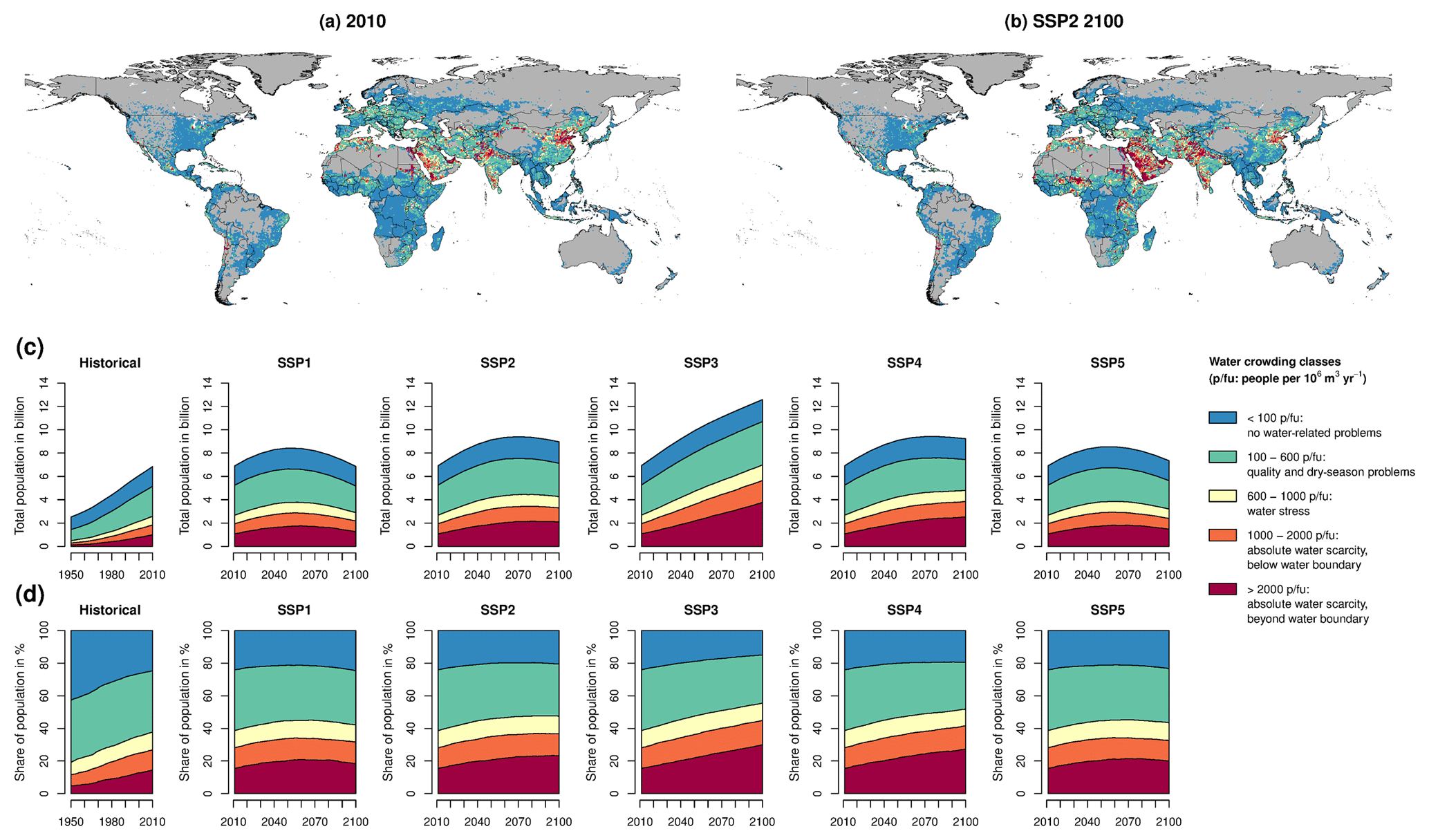
Figure 1Spatial pattern of water crowding in 2010 (a) and in 2100 for SSP2 population (b). Absolute (c) and percentage share of total population (d) in different water crowding classes from 1950 to 2010 and from 2011 to 2100 in five different SSP population scenarios under current water availability, i.e. assuming no climate change.
3.1 Change in water crowding driven by population change
Between 1950 and 2010 the number of people that live with absolute water scarcity (WCI > 1000 p/fu) has increased more than 6 fold from 295 million (11.7 % of global population) to 1.83 billion (26.8 % of global population) due to population growth alone. In the same time period, the number of people beyond the water barrier (WCI > 500 p/fu) within that group has increased more than 8 fold from 118 million (4.7 % of global population) to 988 million people (14.5 % of global population), so that its share within the group of people living under absolute water scarcity has increased from 40.2 % to 53.9 % (Fig. 1c and d).
This trend is projected to continue in the future under all five SSP population scenarios (Fig. 1c and d). The total number of people living under absolute water scarcity in 2100 due to population change alone (without any additional climate change) is projected to be higher than today (2010) in all scenarios reaching 2.16–5.65 billion (31.5 %–44.9 % of global population), with higher global population being associated with higher absolute and relative numbers of affected people. The number of people who live beyond the water barrier is projected to increase to 1.26–3.77 billion (18.4 %–29.9 % of global population, 58.4 %–66.7 % of population under absolute water scarcity).
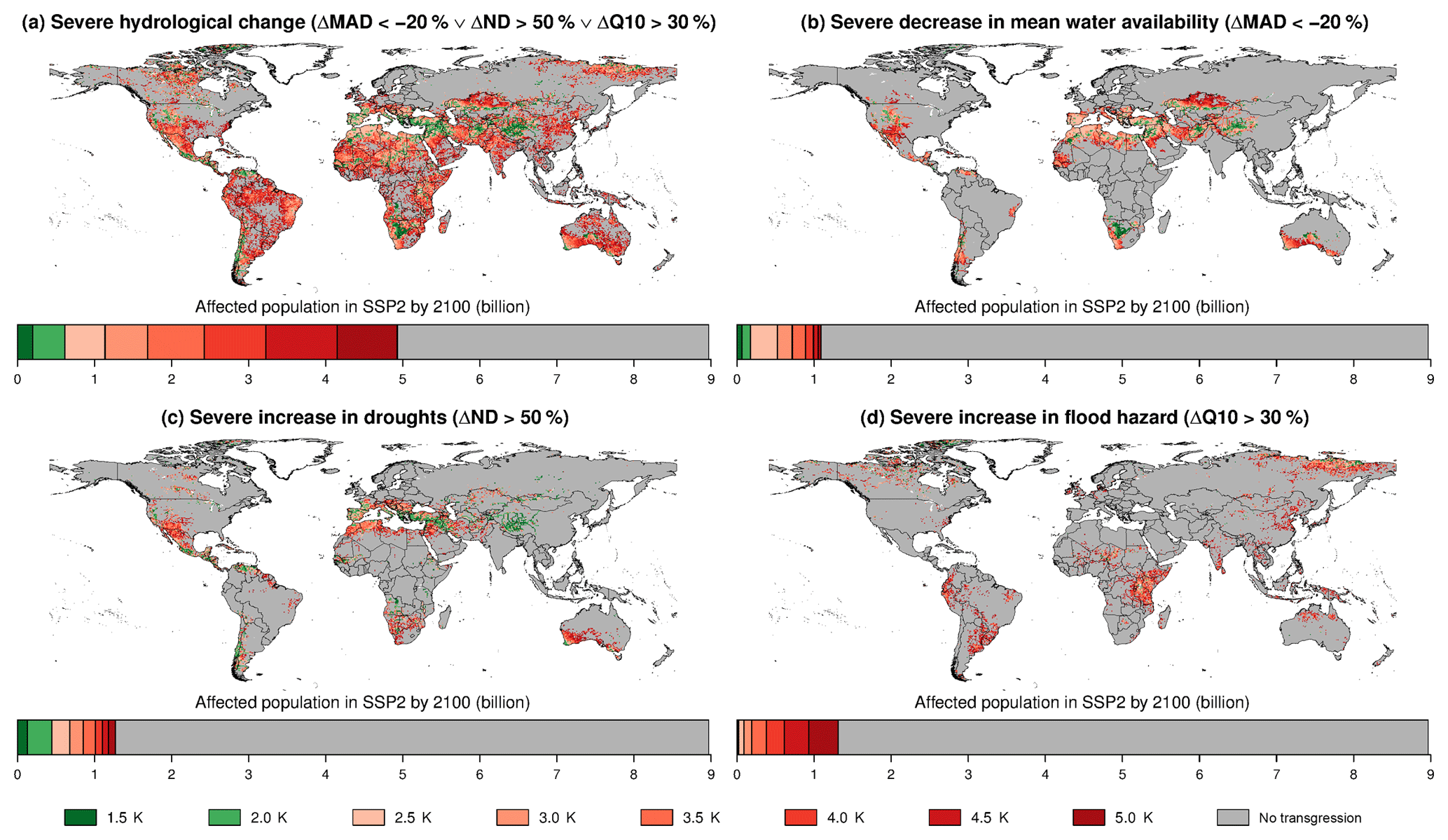
Figure 2ΔTglob at which severe hydrological changes occur in more than half of the GCMs (10 out of 19). Bars underneath the maps indicate population exposed to the respective severe changes for the SSP2 population scenario.
3.2 Severe changes in hydrologic conditions under different levels of ΔTglob
Under the majority of climate change patterns within the range of ΔTglob considered in this study, severe decreases in mean water availability, severe increases in droughts, and severe increases in flood hazard occur in many abundantly populated regions. We estimate that 4.93 billion people (54.9 % of global population) would more likely than not be exposed to severe hydrological change in the SSP2 population scenario if ΔTglob reaches 5 ∘C by 2100 (Fig. 2a; for other SSP scenarios see Supplement Fig. S2). Out of these, 1.09 billion, 1.26 billion, and 1.31 billion would more likely than not be exposed to a severe decrease in mean water availability, a severe increase in droughts, and a severe increase in flood hazard, respectively (Fig. 2b–d). Note that severe decreases in mean water availability and severe increases in droughts often coincide, which leads to relatively large number of people (889 million) being more likely than not exposed to both of these aspects of severe hydrological change. For 2.15 billion people a transgression of the critical threshold for a mix of the three different aspects of severe hydrological change is projected in more than half of the GCMs. The pace at which these levels are reached with increasing ΔTglob is not linear and differs for the three aspects of severe hydrological change. The additional number of people that become exposed to a severe decrease in mean water availability at each step of ΔTglob first increases and then declines again, with the by far largest increment occurring between 2 and 2.5 ∘C. A similar pattern is found for exposure to severe increase in droughts with the difference that the largest increase occurs between 1.5 and 2 ∘C. The increment of people becoming exposed to severe increase in flood hazard is very small until 2 ∘C warming and then steadily increases with ΔTglob. This overall pattern of varying increase in exposure to severe hydrological change with increasing ΔTglob is very similar across all five SSP population scenarios considered here (Fig. S2).
If global warming was limited to 2 ∘C by a successful implementation of the Paris Agreement, the number of people more likely than not exposed to severe hydrological change under SSP2 could be limited to only 615 million people(6.9 % of global population; Fig. 2a), protecting almost 9 out of 10 people (87.5 %) from exposure to severe hydrological change compared to a warming by 5 ∘C. Because exposure to increased flooding hazard remains very low until 2 ∘C warming, the majority of the remaining population would be exposed to severe decreases in mean water availability and severe increases in droughts (Fig. 2b–d). If warming could be limited to 1.5 ∘C the number of people more likely than not exposed to severe hydrological change could be reduced even more to 195 million people (Fig. 2a), a further reduction by more than two-thirds (68.4 %) compared to 2 ∘C warming. However, even a partial failure of the Paris Agreement with an exceedance of the 2∘ target by only 0.5 ∘C would lead to an increase in the number of people exposed to severe hydrological change to 1.14 billion (Fig. 2a) – almost a doubling (84.6 % increase) compared to a warming by 2 ∘C. The main contribution to this strong increase comes from increased exposure to severe decreases in mean water availability and severe increases in droughts, with exposure to severe increases in flood hazard only playing a minor role at these temperature levels (Fig. 2b–d). Although the total number differs across different population scenarios, the percentage of global population that can be protected from exposure to severe hydrological change by ambitious climate mitigation efforts is very similar across all population scenarios (Fig. S2).
3.3 Severe hydrological changes and water scarcity
To get an indication of the adaptation challenges associated with the exposure to severe hydrological change, we use the assessment of future water scarcity due to population change to distinguish two principal adaptation domains. Coping with water scarcity conditions (WCI > 1000 p/fu) even without further aggravation by climate change requires a combination of supply-side and demand-side management measures (Falkenmark, 1989; Ohlsson and Turton, 1999). Therefore, water demand management interventions will also have to play a role in the adaptation to severe hydrological change under already water-scarce conditions. In contrast, adaptation to severe hydrological change under comparatively abundant water availability conditions (WCI ≤1000 p/fu) may be achieved by adjusting water supply infrastructure alone. Although water demand management is generally desirable and may have economic co-benefits (Brooks, 2006), it faces many political, legal, and behavioural obstacles for its implementation and may not be practical in all contexts (Kampragou et al., 2011; Russell and Fielding, 2010).
Under the assumption of no climate change, as much as 3.30 billion people (36.8 % of global population) are estimated to live under absolute water scarcity by 2100 in the SSP2 scenario. For all aspects of severe hydrological change and across the whole range of ΔTglob, the proportion of people more likely than not exposed to severe hydrological change is much larger in this category than in the rest of the population (Fig. 3). This asymmetric distribution of impacts is most pronounced for severe decreases in mean water availability, severe increases in flood hazard, and for severe hydrological change in general (Fig. 3a, c, and d). This finding is largely independent of the population scenario (Fig. S3 in the Supplement).

Figure 3Fraction of SSP2 population in 2100 exposed to severe hydrological change at different levels of ΔTglob (as shown in Fig. 2) divided over two water scarcity categories: population already experiencing absolute water scarcity (> 1000 p/fu) in the absence of climate change and rest of population (≤1000 p/fu). The total number of people in each class is given on the y axis, and the fraction of people exposed to severe hydrological change in each class is given on the x axis. Colour scale for ΔTglob same as in Fig. 2.
Because of the challenges associated with the implementation of demand-side management interventions, the population already experiencing water scarcity in the absence of climate change is of primary concern when analysing exposure to severe hydrological change. We estimate that 2.14 billion people (23.9 % of global population) in the SSP2 population scenario would be affected by water scarcity due to population change and more likely than not exposed to climate-related severe hydrological change if ΔTglob would rise to 5 ∘C by 2100 (Fig. 3a). Out of these, 538 million (6.0 % of global population), 500 million (5.7 % of global population), and 640 million (7.1 % of global population) would more more likely than not be exposed to a severe decrease in mean water availability, a severe increase in droughts, and a severe increase in flood hazard, respectively (Fig. 3b–d). For 875 million people, a transgression of thresholds for a mix of different aspects of severe hydrological change is found in more than half of the GCMs. A successful implementation of the Paris Agreement that would limit warming to 2 ∘C would dramatically reduce the number of people under absolute water scarcity and more likely than not exposed to severe hydrological change to 290 million (3.2 % of global population). With even more ambitious mitigation efforts sufficient to limit warming to 1.5 ∘C warming could further reduce this number to as little as 116 million people (1.3 % of global population). For a failure of the Paris Agreement with temperature rising to 2.5 ∘C (3 ∘C) this number would rise to 543 (824) million people.
Table 1Number of people in 2100 for the SSP2 population scenario that would experience absolute water scarcity (> 1000 p/fu) under present-day climate conditions and be more likely than not exposed to severe hydrological change at different levels of ΔTglob in different world regions (population in million, percentage of population in region in brackets). Regions are MEA (Middle East and north Africa), ANZ (Australia and New Zealand), SAS (South Asia), SSA (sub-Saharan Africa), LAM (Latin America), NAM (USA and Canada), EUR (Europe, excluding Russia), EAS (East Asia), RCA (Russia and Central Asia), and SEA (Southeast Asia).
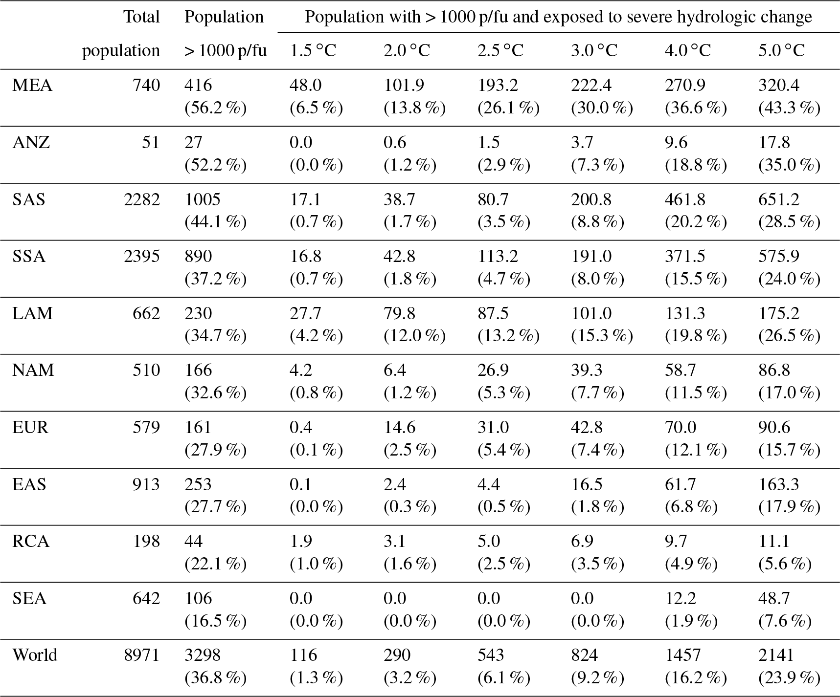
The remaining number of people exposed to severe hydrological change at 2 ∘C warming, as well as the implications of more ambitious mitigation efforts or a failure of the Paris Agreement, differs greatly among world regions (Table 1, for countries assigned to each region see Fig. S4). About 63 % of the 290 million people who live under absolute water scarcity and are more likely than not exposed to severe hydrologic change at 2 ∘C warming live in Latin America (LAM) and the Middle East and north Africa region (MEA), where they make up more than 12 % of the population in those regions. Another 28 % of the 290 million live in South Asia (SAS) and sub-Saharan Africa (SSA), but due to high population numbers in these regions their share remains below 2 %. The high share of population affected by absolute water scarcity and severe hydrological change in LAM and MEA is particularly worrying since a failure to overcome the obstacles associated with the implementation of appropriate demand management can have negative societal and economic consequences not only for these people but for the whole region. More ambitious mitigation efforts that keep warming below 1.5 ∘C would reduce the number of affected people by more than half, to 6.5 % in MEA and 4.2 % in LAM. In all other regions, the share of affected population would drop below 1 %.
Failure of the Paris Agreement would substantially increase exposure to severe hydrological change in many regions. In 5 out of 10 regions, the number of people affected by absolute water scarcity and severe hydrological change at least doubles if the 2 ∘C target is exceeded by only 0.5 ∘C and reaches a share of (almost) 5 % of affected population in the region in SSA, North America (NAM), and Europe (EUR). The strongest absolute increase (though not a doubling) in the number of affected people occurs in the MEA region, where more than one-quarter of the population in that region would be affected at 2.5 ∘C warming. Between 2.5 and 3 ∘C warming, the increases in number of affected people is strongest in South Asia (SAS), SSA, NAM, and EUR. At 4 ∘C warming, the share of affected population exceeds 10 % in 7 out of 10 regions, with MEA, Australia and New Zealand (ANZ), SAS, SSA, and LAM being most strongly impacted. At 5 ∘C warming, the share of affected population reaches 43.3 % in MEA and 35.0 % in ANZ; exceeds 20 % in SAS, SSA, and LAM; and exceeds 15 % in NAM, EUR, and East Asia (EAS). In Russia and Central Asia (RCA) and Southeast Asia (SEA) the share of affected people remains below 5 %, partly due to a low share of population under high water crowding and less severe hydrologic change.
Although numbers differ among population scenarios, the overall pattern of where and how much change occurs in the different regions is consistent across all SSP population scenarios. A comprehensive overview of population under high water crowding and affected by severe hydrologic change in different world regions for all population scenarios is given in Fig. S5.
Our estimate that 26.8 % of global population today live under absolute water scarcity (> 1000 p/fu) is within the range of 21.0 %–27.5 % (average 24.7 %) reported by previous studies applying the WCI on river basin level (Gerten et al., 2013; Arnell and Lloyd-Hughes, 2014; Kummu et al., 2016). Estimates of future SSP populations living in river basins with > 1000 p/fu under present-day climate conditions are given by Arnell and Lloyd-Hughes (2014) who estimate a range of 39.5 %–54.2 % for the affected global population across different SSP scenarios. This is considerably higher than the range of our estimates of 31.5 %–44.9 %; but due to the lack of other comparable studies, it is not clear whether these discrepancies are caused by the choice of the hydrological model or by the difference in scale (basin or grid cell) at which the WCI is calculated. However, using the same hydrological model as in our study, Gerten et al. (2013) estimate that 38.5 % of global population in the revised A2r scenario (Grübler et al., 2007) from the Special Report on Emissions Scenarios would live in river basins with > 1000 p/fu under current climate conditions, which is close to our estimate of 41.0 % for the SSP3 scenario, to which the A2r scenario is comparable in terms of total population (12.3 billion compared to 12.6 billion in 2100). In contrast, the corresponding estimate by Arnell and Lloyd-Hughes (2014) is as high as 54.2 % for the SSP3 scenario, which indicates that using LPJmL to assess water scarcity generally tends to result in lower estimates of future population affected by water scarcity.
A direct comparison of hydrological changes estimated here to previous studies is not straightforward due to the unique design of this study. Only few global studies have assessed climate change impacts on water resources as a function of ΔTglob (Gerten et al., 2013; Schewe et al., 2014; Gosling and Arnell, 2016), but they typically focus on changes in MAD and report changes in the number of people affected by water scarcity. A relevant study for comparison is Schewe et al. (2014), which analyses changes in MAD obtained from an ensemble of 10 global hydrological models (GHMs) forced by climate scenarios from five different GCMs. The overall pattern of changes in MAD simulated by LPJmL across 19 GCMs agrees well with results from Schewe et al. (2014), but exhibits a generally lower magnitude of changes (see Fig. S6 and Fig. 1 in Schewe et al., 2014). Thus, MAD changes simulated by LPJmL (both increases and decreases) tend to be smaller than simulated by most other GHMs. This becomes even more apparent when comparing the percentage of people affected by a 20 % decrease in MAD. For a ΔTglob of 2.5 ∘C (equivalent to an additional warming of 1.9 ∘C relative to the control simulation) we estimate a median share of 8.6 % of affected global population across all GCMs. This is substantially lower than the median value of 13 % of affected population estimated for 2 ∘C additional warming by Schewe et al. (2014) and approximately represents their lower end of the interquartile range. This can be attributed to the response of dynamic vegetation in LPJmL that is not included in most other GHMs (Schewe et al., 2014).
In summary, the global and regional estimates of population living under absolute water scarcity and being exposed to severe hydrological change obtained from LPJmL are lower than from most other GHMs. Thus, the estimates of population affected by water scarcity and severe hydrological change presented in this paper should be regarded as conservative estimates.
Apart from these uncertainties in model projections, the results of a global study like ours are necessarily determined by simplifications and generalization in the data analysis. The most important generalization in this study are the choice of aspects of severe hydrological change and the corresponding critical thresholds. While not all selected aspects may be relevant in all cases (e.g. where supply is primarily fulfilled from groundwater), we believe that in the vast majority of cases they reflect important hydrological properties that are relevant from a freshwater resource perspective. The respective thresholds may also differ depending on hydrological and other local conditions, and using unique global values will always produce a number of false positives and false negatives. However, the selected thresholds are rather conservative, and thus are expected to produce more false negatives than false positives. Another aspect is the choice of the WCI to differentiate population groups in terms of adaptation challenges. This indicator is widely applied because it only requires data on mean water availability and population numbers, but it can neither account for hydrological aspects that limit the utilization of water resources nor for actual per capita water requirements. Despite these shortcomings of the WCI, it gives a rough impression of the overall population pressure on water resources, which is linked to the challenges to adapt to severe hydrological change. Last but not least, it is important to note that this study only addresses quantity aspects of freshwater resources and does not consider water quality.
Future freshwater supply will be affected by population growth and climate change, which are both subject to uncertainty and heterogeneous distribution patterns. Under all five SSP population projections considered here, a strong increase in the number of people living under absolute water scarcity in 2100 to 2.16–5.65 billion (31.5 %–44.9 % of global population) is projected, with higher global population resulting in higher absolute numbers but also larger proportions of global population being affected. Because of the importance of water demand management for coping with absolute water scarcity, which is more difficult to implement than supply management, these parts of the global population will face higher challenges for adaption to severe hydrological change that affects water supply.
If global warming would continue unabated to reach 5 ∘C above pre-industrial levels in 2100, 4.93 billion people (54.9 % of global population) in the SSP2 population scenario would more likely than not be exposed to severe hydrological change. Out of those, 2.14 billion people (23.9 % of global population) would already experience absolute water scarcity due to high population pressure on water resources, making adaptation to such changes more challenging. With a successful implementation of the Paris Agreement limiting global warming to 2 ∘C, the number of people affected by severe hydrological change could be reduced to 615 million people (6.9 % of global population), of which 290 million (3.2 % of global population) would already experience absolute water scarcity. If temperature increase could be limited to 1.5 ∘C, the number of people exposed to severe hydrological change could be further reduced to 195 million (2.2 %) and 116 million (1.3 %), respectively. However, only a partial failure of the Paris Agreement with temperature rising to 2.5 ∘C would almost double the number of people more likely than not exposed to severe hydrological change, in total and among those already experiencing absolute water scarcity, compared to a 2 ∘C warming.
Due to the heterogeneous spatial distribution of absolute water scarcity and severe hydrological change, the proportion of population exposed to severe hydrological change with increased adaption challenges reaches 12.0 % in Latin America and 13.8 % in the Middle East and north Africa region even if global warming could be limited 2 ∘C by a successful implementation of the Paris Agreement. A failure to overcome the obstacles associated with the implementation of appropriate demand management can have negative societal and economic consequences not only for these people but for the whole region. Thus, 2 ∘C mean global warming cannot be considered a safe limit of warming in these regions. More ambitious mitigation efforts that would keep warming at, or below, 1.5 ∘C could substantially reduce that risk by reducing the share of population exposed to severe hydrological change and with increased adaption challenges by more than half in these two regions and globally.
The CRU TS3.1 historical climate data are available from http://catalogue.ceda.ac.uk/uuid/ac3e6be017970639a9278e64d3fd5508 (University of East Anglia Climatic Research Unit, Jones, and Harris, 2013). The temperature-stratified climate scenarios of the PanClim dataset along with the matched GPCC historical precipitation data are available from http://www.panclim.org (Heinke et al., 2013b). Historic gridded population estimates up to the year 2010 are based on the Gridded Population of the World, Version 3 (GPWv3) Data Collection (CIESIN-CIAT, 2005), which have been edited and provided by the Inter-Sectoral Impact Model Intercomparison Project (ISIMIP, 2012; Warszawski et al., 2014). The gridded historical population data are available from https://www.isimip.org/gettingstarted/details/13/ (CIESIN-CIAT, 2005) and the future scenario population data are available from https://doi.org/10.7927/H4RF5S0P (Jones and O'Neill, 2017). The STN-30p flow direction map can be downloaded from https://doi.org/10.3334/ORNLDAAC/1005 (Vörsömarty et al., 2011). The model code of LPJmL4 is publicly available from https://doi.org/10.5880/pik.2018.002 (Schaphoff et al., 2018c) or via the GitHub project page https://github.com/PIK-LPJmL/LPJmL (last access: 5 February 2019). The core output of the analysis in this paper-consisting of historic and future scenario water crowding estimates as well as hydrological indicators for 19 GCMs an 8 levels of global mean temperature increase at 0.5∘ resolution-has been made available under a Creative Commons Attribution 4.0 License and is available for download from https://doi.org/10.5281/zenodo.2562056 (Heinke et al., 2019). All results presented in this paper are based on this core output. All primary data, model code, model outputs and scripts that have been used to produce the core output and the results presented in this paper are archived at the Potsdam Institute for Climate Impact Research and are available upon request.
The supplement related to this article is available online at: https://doi.org/10.5194/esd-10-205-2019-supplement.
WL and DG formulated the overarching research goal; JH designed the study, performed all model runs, and carried out the analysis; JH, CM, and ML discussed results; JH wrote the manuscript with contributions from all co-authors.
The authors declare that they have no conflict of interest.
This article is part of the special issue “The Earth system at a global warming of 1.5 ∘C and 2.0 ∘C”. It is not associated with a conference.
This work was in part supported by German Federal Ministry of Education and
Research (BMBF) through the project SUSTAg (031B0170A). The authors would
like to thank the two anonymous referees for helpful comments on the
manuscript.
The article
processing charges for this open-access
publication were covered by the Potsdam Institute
for Climate Impact Research (PIK).
Edited by: Rolf Aalto
Reviewed by: two anonymous referees
Arnell, N. W.: Climate change and global water resources: SRES emissions and socio-economic scenarios, Glob. Environ. Chang., 14, 31–52, https://doi.org/10.1016/j.gloenvcha.2003.10.006, 2004.
Arnell, N. W. and Lloyd-Hughes, B.: The global-scale impacts of climate change on water resources and flooding under new climate and socio-economic scenarios, Clim. Change, 122, 127–140, https://doi.org/10.1007/s10584-013-0948-4, 2014.
Brooks, D. B.: An Operational Definition of Water Demand Management, Int. J. Water Resour. Dev., 22, 521–528, https://doi.org/10.1080/07900620600779699, 2006.
CIESIN-CIAT (Center for International Earth Science Information Network): Columbia University, Centro Internacional de Agricultura Tropical (CIAT): Gridded Population of the World, Version 3 (GPWv3), NASA Socioeconomic Data and Applications Center (SEDAC), Palisades, NY, available at: http://sedac.ciesin.columbia.edu/data/collection/gpw-v3/ (last access: 5 February 2019), 2005.
Coles, S.: An Introduction to Statistical Modeling of Extreme Values, Springer London, London, 2001.
Dankers, R., Arnell, N. W., Clark, D. B., Falloon, P. D., Fekete, B. M., Gosling, S. N., Heinke, J., Kim, H., Masaki, Y., Satoh, Y., Stacke, T., Wada, Y., and Wisser, D.: First look at changes in flood hazard in the Inter-Sectoral Impact Model Intercomparison Project ensemble, P. Natl. Acad. Sci. USA, 111, 3257–3261, https://doi.org/10.1073/pnas.1302078110, 2013.
Döll, P. and Schmied, H. M.: How is the impact of climate change on river flow regimes related to the impact on mean annual runoff? A global-scale analysis, Environ. Res. Lett., 7, 014037, https://doi.org/10.1088/1748-9326/7/1/014037, 2012.
Dyck, S. and Peschke, G.: Grundlagen der Hydrologie, 3rd ed., Verlag für Bauwesen, Berlin, 1995.
Fader, M., Rost, S., Müller, C., Bondeau, A., and Gerten, D.: Virtual water content of temperate cereals and maize: Present and potential future patterns, J. Hydrol., 384, 218–231, https://doi.org/10.1016/j.jhydrol.2009.12.011, 2010.
Falkenmark, M.: The Massive Water Scarcity Now Threatening Africa – Why Isn't It Being Addressed, Ambio, 18, 112–118, 1989.
Falkenmark, M. and Lannerstad, M.: Consumptive water use to feed humanity – curing a blind spot, Hydrol. Earth Syst. Sci., 9, 15–28, https://doi.org/10.5194/hess-9-15-2005, 2005.
Gerten, D., Heinke, J., Hoff, H., Biemans, H., Fader, M., and Waha, K.: Global Water Availability and Requirements for Future Food Production, J. Hydrometeorol., 12, 885–899, https://doi.org/10.1175/2011JHM1328.1, 2011.
Gerten, D., Lucht, W., Ostberg, S., Heinke, J., Kowarsch, M., Kreft, H., Kundzewicz, Z. W., Rastgooy, J., Warren, R., and Schellnhuber, H. J.: Asynchronous exposure to global warming: freshwater resources and terrestrial ecosystems, Environ. Res. Lett., 8, 034032, https://doi.org/10.1088/1748-9326/8/3/034032, 2013.
Gosling, S. N. and Arnell, N. W.: A global assessment of the impact of climate change on water scarcity, Clim. Change, 134, 371–385, https://doi.org/10.1007/s10584-013-0853-x, 2016.
Grübler, A., O'Neill, B., Riahi, K., Chirkov, V., Goujon, A., Kolp, P., Prommer, I., Scherbov, S., and Slentoe, E.: Regional, national, and spatially explicit scenarios of demographic and economic change based on SRES, Technol. Forecast. Soc. Change, 74, 980–1029, https://doi.org/10.1016/j.techfore.2006.05.023, 2007.
Harris, I., Jones, P. D., Osborn, T. J., and Lister, D. H.: Updated high-resolution grids of monthly climatic observations – the CRU TS3.10 Dataset, Int. J. Climatol., 34, 623–642, https://doi.org/10.1002/joc.3711, 2014.
Heinke, J., Ostberg, S., Schaphoff, S., Frieler, K., Müller, C., Gerten, D., Meinshausen, M., and Lucht, W.: A new climate dataset for systematic assessments of climate change impacts as a function of global warming, Geosci. Model Dev., 6, 1689–1703, https://doi.org/10.5194/gmd-6-1689-2013, 2013a.
Heinke, J., Ostberg, S., Schaphoff, S., Frieler, K., Müller, C., Gerten, D., Meinshausen, M., and Lucht, W.: PanClim future climate scenarios: PanClim: A new climate dataset for systematic assessments of climate change impacts as a function of global warming, available at: http://www.panclim.org (last access: 5 February 2019), 2013b.
Heinke, J., Müller, C., Lannerstad, M., Gerten, D., and Lucht, W.: Core output: Freshwater resources under success and failure of the Paris climate agreement [Data set], Zenodo, https://doi.org/10.5281/zenodo.2562056, 2019.
Hosking, J. R. M. and Wallis, J. R.: A Comparison of Unbiased and Plotting-Position Estimators of L Moments, Water Resour. Res., 31, 2019–2025, https://doi.org/10.1029/95WR01230, 1995.
International Council for Science (ICSU): A Guide to SDG Interactions: from Science to Implementation, edited by: Griggs, D. J., Nilsson, M., Stevance, A., and McCollum, D., International Council for Science, Paris, 2017.
ISIMIP (Inter-Sectoral Impact Model Intercomparison Project): Population & GDP, available at: https://www.isimip.org/gettingstarted/details/13/ (last access: 5 February 2019), 2012.
Jägermeyr, J., Gerten, D., Schaphoff, S., Heinke, J., Lucht, W., and Rockström, J.: Integrated crop water management might sustainably halve the global food gap, Environ. Res. Lett., 11, 025002, https://doi.org/10.1088/1748-9326/11/2/025002, 2016.
Jones, B. and O'Neill, B. C.: Spatially explicit global population scenarios consistent with the Shared Socioeconomic Pathways, Environ. Res. Lett., 11, 084003, https://doi.org/10.1088/1748-9326/11/8/084003, 2016.
Jones, B. and O'Neill, B. C.: Global Population Projection Grids Based on Shared Socioeconomic Pathways (SSPs), 2010–2100, NASA Socioeconomic Data and Applications Center (SEDAC), Palisades, NY, https://doi.org/10.7927/H4RF5S0P (last access: 5 February 2019), 2017.
Kampragou, E., Lekkas, D. F., and Assimacopoulos, D.: Water demand management: implementation principles and indicative case studies, Water Environ. J., 25, 466–476, https://doi.org/10.1111/j.1747-6593.2010.00240.x, 2011.
KC, S. and Lutz, W.: The human core of the shared socioeconomic pathways: Population scenarios by age, sex and level of education for all countries to 2100, Glob. Environ. Chang., 42, 181–192, https://doi.org/10.1016/j.gloenvcha.2014.06.004, 2017.
Kummu, M., Guillaume, J. H. A., de Moel, H., Eisner, S., Flörke, M., Porkka, M., Siebert, S., Veldkamp, T. I. E., and Ward, P. J.: The world's road to water scarcity: shortage and stress in the 20th century and pathways towards sustainability, Sci. Rep., 6, 38495, https://doi.org/10.1038/srep38495, 2016.
Mastrandrea, M. D., Mach, K. J., Plattner, G.-K., Edenhofer, O., Stocker, T. F., Field, C. B., Ebi, K. L., and Matschoss, P. R.: The IPCC AR5 guidance note on consistent treatment of uncertainties: a common approach across the working groups, Clim. Change, 108, 675–691, https://doi.org/10.1007/s10584-011-0178-6, 2011.
Meinshausen, M., Raper, S. C. B., and Wigley, T. M. L.: Emulating coupled atmosphere-ocean and carbon cycle models with a simpler model, MAGICC6 – Part 1: Model description and calibration, Atmos. Chem. Phys., 11, 1417–1456, https://doi.org/10.5194/acp-11-1417-2011, 2011.
O'Neill, B. C., Kriegler, E., Ebi, K. L., Kemp-Benedict, E., Riahi, K., Rothman, D. S., van Ruijven, B. J., van Vuuren, D. P., Birkmann, J., Kok, K., Levy, M., and Solecki, W.: The roads ahead: Narratives for shared socioeconomic pathways describing world futures in the 21st century, Glob. Environ. Chang., 42, 169–180, https://doi.org/10.1016/j.gloenvcha.2015.01.004, 2017.
Ohlsson, L. and Turton, A. R.: The turning of a screw: Social resource scarcity as a bottleneck in adaptation to water scarcity, Occasional Paper Series, School of Oriental and African Studies, Water Study Group, University of London, 1999.
Raskin, P. D., Hansen, E., and Margolis, R. M.: Water and sustainability, Nat. Resour. Forum, 20, 1–15, https://doi.org/10.1111/j.1477-8947.1996.tb00629.x, 1996.
Rockström, J., Falkenmark, M., Folke, C., Lannerstad, M., Barron, J., Enfors, E., Gordon, L., Heinke, J., Hoff, H., and Pahl-Wostl, C.: Water Resilience for Human Prosperity, Cambridge University Press, Cambridge, UK, 2014.
Rogelj, J., den Elzen, M., Höhne, N., Fransen, T., Fekete, H., Winkler, H., Schaeffer, R., Sha, F., Riahi, K., and Meinshausen, M.: Paris Agreement climate proposals need a boost to keep warming well below 2 ∘C, Nature, 534, 631–639, https://doi.org/10.1038/nature18307, 2016.
Rost, S., Gerten, D., Bondeau, A., Lucht, W., Rohwer, J., and Schaphoff, S.: Agricultural green and blue water consumption and its influence on the global water system, Water Resour. Res., 44, 1–17, https://doi.org/10.1029/2007WR006331, 2008.
Russell, S. and Fielding, K.: Water demand management research: A psychological perspective, Water Resour. Res., 46, 1–12, https://doi.org/10.1029/2009WR008408, 2010.
Schaphoff, S., von Bloh, W., Rammig, A., Thonicke, K., Biemans, H., Forkel, M., Gerten, D., Heinke, J., Jägermeyr, J., Knauer, J., Langerwisch, F., Lucht, W., Müller, C., Rolinski, S., and Waha, K.: LPJmL4 – a dynamic global vegetation model with managed land – Part 1: Model description, Geosci. Model Dev., 11, 1343–1375, https://doi.org/10.5194/gmd-11-1343-2018, 2018a.
Schaphoff, S., Forkel, M., Müller, C., Knauer, J., von Bloh, W., Gerten, D., Jägermeyr, J., Lucht, W., Rammig, A., Thonicke, K., and Waha, K.: LPJmL4 – a dynamic global vegetation model with managed land – Part 2: Model evaluation, Geosci. Model Dev., 11, 1377–1403, https://doi.org/10.5194/gmd-11-1377-2018, 2018b.
Schaphoff, S. (Ed.), von Bloh, W., Thonicke, K., Biemans, H., Forkel, M., Gerten, D., Heinke, J., Jägermeyr, J., Müller, C., Rolinski, S., Waha, Ka., Stehfest, E., de Waal, L., Heyder, U., Gumpenberger, M., and Beringer, T.: LPJmL4 Model Code, V. 4.0, GFZ Data Services, https://doi.org/10.5880/pik.2018.002 (last access: 5 February 2019), 2018c.
Schewe, J., Heinke, J., Gerten, D., Haddeland, I., Arnell, N. W., Clark, D. B., Dankers, R., Eisner, S., Fekete, B. M., Colón-González, F. J., Gosling, S. N., Kim, H., Liu, X., Masaki, Y., Portmann, F. T., Satoh, Y., Stacke, T., Tang, Q., Wada, Y., Wisser, D., Albrecht, T., Frieler, K., Piontek, F., Warszawski, L., and Kabat, P.: Multimodel assessment of water scarcity under climate change, P. Natl. Acad. Sci. USA, 111, 3245–3250, https://doi.org/10.1073/pnas.1222460110, 2014.
Schneider, U., Becker, A., Finger, P., Meyer-Christoffer, A., Ziese, M., and Rudolf, B.: GPCC's new land surface precipitation climatology based on quality-controlled in situ data and its role in quantifying the global water cycle, Theor. Appl. Climatol., 115, 15–40, https://doi.org/10.1007/s00704-013-0860-x, 2014.
Steffen, W., Richardson, K., Rockstrom, J., Cornell, S. E., Fetzer, I., Bennett, E. M., Biggs, R., Carpenter, S. R., de Vries, W., de Wit, C. A., Folke, C., Gerten, D., Heinke, J., Mace, G. M., Persson, L. M., Ramanathan, V., Reyers, B., and Sorlin, S.: Planetary boundaries: Guiding human development on a changing planet, Science, 347, 6223, https://doi.org/10.1126/science.1259855, 2015.
UNFCCC: Paris Agreement: FCCC/CP/2015/L.9/Rev.1, available at: http://unfccc.int/resource/docs/2015/cop21/eng/l09r01.pdf (last access: 5 February 2019), 2015.
United Nations: Transforming our world: The 2030 agenda for sustainable development, UN General Assembly, New York, available at: https://sustainabledevelopment.un.org/post2015/transformingourworld (last access: 5 February 2019), 2015.
United Nations: The Sustainable Development Goals Report 2017, United Nations, 2017.
University of East Anglia Climatic Research Unit, Jones, P. D., and Harris, I. C.: CRU TS3.10: Climatic Research Unit (CRU) Time-Series (TS) Version 3.10 of High Resolution Gridded Data of Month-by-month Variation in Climate (Jan 1901–Dec 2009), NCAS British Atmospheric Data Centre, available at: http://catalogue.ceda.ac.uk/uuid/ac3e6be017970639a9278e64d3fd5508 (last access: 5 February 2019), 2013.
van Huijgevoort, M. H. J., Hazenberg, P., van Lanen, H. A. J., and Uijlenhoet, R.: A generic method for hydrological drought identification across different climate regions, Hydrol. Earth Syst. Sci., 16, 2437–2451, https://doi.org/10.5194/hess-16-2437-2012, 2012.
Victor, D. G., Akimoto, K., Kaya, Y., Yamaguchi, M., Cullenward, D., and Hepburn, C.: Prove Paris was more than paper promises, Nature, 548, 25–27, https://doi.org/10.1038/548025a, 2017.
Vörösmarty, C. J., Fekete, B. M., Meybeck, M., and Lammers, R. B.: Global system of rivers: Its role in organizing continental land mass and defining land-to-ocean linkages, Global Biogeochem. Cy., 14, 599–621, https://doi.org/10.1029/1999GB900092, 2000.
Vörösmarty, C. J., Fekete, B. M., Hall, F. G., Collatz, G. J., Meeson, B. W., Los, S. O., Brown De Colstoun, E., and Landis, D. R.: ISLSCP II River Routing Data (STN-30p), ORNL DAAC, Oak Ridge, Tennessee, USA, https://doi.org/10.3334/ORNLDAAC/1005 (last access: 5 February 2019), 2011.
Warszawski, L., Frieler, K., Huber, V., Piontek, F., Serdeczny, O., and Schewe, J.: The Inter-Sectoral Impact Model Intercomparison Project (ISI-MIP): Project framework, Proc. Natl. Acad. Sci. USA, 111, 3228–3232, https://doi.org/10.1073/pnas.1312330110, 2014.