On the future role of the most parsimonious  climate module in integrated assessment

Khabbazan, Mohammad M.; Held, Hermann

doi:https://doi.org/10.5194/esd-10-135-2019

Articles | Volume 10, issue 1

https://doi.org/10.5194/esd-10-135-2019

Articles | Volume 10, issue 1

Research article

14 Mar 2019

Research article |

| 14 Mar 2019

On the future role of the most parsimonious climate module in integrated assessment

Mohammad M. Khabbazan and Hermann Held

Abstract

In the following, we test the validity of a one-box climate model as an emulator for atmosphere–ocean general circulation models (AOGCMs). The one-box climate model is currently employed in the integrated assessment models FUND, MIND, and PAGE, widely used in policy making. Our findings are twofold. Firstly, when directly prescribing AOGCMs' respective equilibrium climate sensitivities (ECSs) and transient climate responses (TCRs) to the one-box model, global mean temperature (GMT) projections are generically too high by 0.5 K at peak temperature for peak-and-decline forcing scenarios, resulting in a maximum global warming of approximately 2 K. Accordingly, corresponding integrated assessment studies might tend to overestimate mitigation needs and costs. We semi-analytically explain this discrepancy as resulting from the information loss resulting from the reduction of complexity. Secondly, the one-box model offers a good emulator of these AOGCMs (accurate to within 0.1 K for Representative Concentration Pathways, RCPs, namely RCP2.6, RCP4.5, and RCP6.0), provided the AOGCM's ECS and TCR values are universally mapped onto effective one-box counterparts and a certain time horizon (on the order of the time to peak radiative forcing) is not exceeded. Results that are based on the one-box model and have already been published are still just as informative as intended by their respective authors; however, they should be reinterpreted as being influenced by a larger climate response to forcing than intended.

Download & links

Article (PDF, 4624 KB)

Download & links

How to cite.

Received: 04 Apr 2017 – Discussion started: 09 May 2017 – Revised: 15 Jan 2019 – Accepted: 21 Feb 2019 – Published: 14 Mar 2019

1 Introduction

Climate–economy integrated assessment models (IAMs) are used to derive welfare-optimal climate policy scenarios (Kunreuther et al., 2014) or constrained welfare-optimal scenarios that comply with a prescribed policy target (Clarke et al., 2014). Most of them employ relatively simple climate modules emulating sophisticated climate models, atmosphere–ocean general circulation models (AOGCMs). These climate modules (hereafter “simple climate models” – SCMs) offer computational efficiency and hence allow researchers to examine a broader set of scenarios in orders of magnitude less time. For IAMs based on a decision-analytic framework involving intertemporal welfare optimization, SCMs are in fact indispensable, as these IAMs' numerical solvers may need to access the climate module anywhere from 10 000 to 100 000 times before numerical convergence is flagged.

The need to qualify the degree of accuracy with which SCMs mimic AOGCMs or properly represent ensembles of AOGCMs is increasingly being recognized (Calel and Stainforth, 2017; van Vuuren et al., 2011a), as this aspect might have immediate monetary consequences in connection with derived policy scenarios (Calel and Stainforth, 2017). In previous work, van Vuuren et al. (2011a) found that IAMs tend to underestimate the effects of greenhouse gas emissions.

Due to the centennial-scale quasi-linear properties of AOGCMs' global mean temperature (GMT) dynamics, SCMs have proven capable of emulating AOGCMs' behavior regarding GMT change, with deviations being a function of spread of forcing, SCM complexity (Meinshausen et al., 2011a), and quality of SCM calibration. The climate component of the Model for the Assessment of Greenhouse Gas Induced Climate Change (MAGICC; Meinshausen et al., 2011a) represents the most complex SCM currently in use. In some sense one could even call MAGICC an Earth system model of intermediate complexity. It has demonstrated its capacity to emulate all AOGCMs' GMT even more precisely than the standard deviation of interannual GMT variability (Meinshausen et al., 2011a), with a fixed set of parameters, utilized for the whole range of Representative Concentration Pathways (RCPs) (see van Vuuren et al., 2011b). This represents the current gold standard of AOGCM emulation using SCMs.

The most extreme opposite end of the scale of complexity within the model category of SCMs is provided by the one-box model as introduced by Petschel-Held et al. (1999) (hereafter “PH99”), converting a radiative forcing time series into a GMT time series. The current role of this model as assessed in the literature is as follows: by fitting PH99 to GMT time series, it can be used as a diagnostic instrument, as Andrews and Allen (2008) have done. However, its main application is as an emulator of AOGCMs. In conjunction with the most parsimonious carbon cycle model (described in Petschel-Held et al., 1999 as well), PH99 has been used to derive “admissible” greenhouse gas emission scenarios in view of prescribed GMT targets (Bruckner et al., 2003; Kriegler and Bruckner, 2004). Furthermore, the following climate–economic IAMs are currently utilizing PH99: FUND (Anthoff and Tol, 2014), MIND (Edenhofer et al., 2005), and PAGE (Hope, 2006) – the last of which was used in the “Stern Review” for the UK government (Stern, 2007). While MIND has since been succeeded by the IAM REMIND (Luderer et al., 2011) when it comes to spatial resolution or representing the energy sector by dozens of technologies, it currently serves as a state-of-the-art IAM for decision-making under uncertainty (Held et al., 2009; Lorenz et al., 2012; Neubersch et al., 2014; Roth et al., 2015) or joint mitigation–solar radiation management analyses (Roshan et al., 2019; Stankoweit et al., 2015).

Kriegler and Bruckner (2004) validated PH99 in conjunction with a simple carbon cycle model. When diagnosing the effect of the IS92a emissions scenario (Kattenberg et al., 1996) on GMT, they demonstrated deviations of less than 0.2 K for the 21st century (see their Fig. 5). Recently, Calel and Stainforth (2017) highlighted the potential future role of PH99 and hence further validation of its behavior is warranted.

In this article, we ask by what calibration procedure is PH99's temperature response to radiative forcing able to correctly map globally averaged radiative forcing anomalies onto GMT anomalies? In this article, “correctly” refers to an accuracy on the order of magnitude of the standard deviation of natural variability, i.e., ∼0.1 K. Furthermore, in the context of this article we would judge a deviation of 0.5 K as inacceptable because a proclaimed goal of the 2015 Paris Agreement (UNFCCC, 2016) is “… holding the increase in the global average temperature to well below 2 ^∘C above preindustrial levels and pursuing efforts to limit the temperature increase to 1.5 ^∘C above preindustrial levels …” In the policy domain, a difference of 0.5 K matters.

We believe that further validation of PH99 is necessary and possible, at a higher level of consistency than has been performed previously. Firstly, the respective GMT time series as checked in Kriegler and Bruckner (2004) is convexly increasing. However in the context of scenario generation in keeping with the well-below 2 K target (UNFCCC, 2016), validation along GMT stabilization or even peaking scenarios is crucial, as these scenarios display a qualitatively different shape from IS92a. Secondly, in Kattenberg et al. (1996) the forcing was reconstructed by the additional assumption that non-CO₂ greenhouse gas forcing approximately balances aerosol cooling.

Here we employ recently diagnosed forcings for 14 CMIP5 AOGCMs by Forster et al. (2013). As a main finding we diagnose that in the context of 2 K stabilization scenarios, it would be necessary to implement a smaller equilibrium climate sensitivity (ECS) value in PH99 than the diagnosed ECS value of the very AOGCM which PH99 is supposed to emulate. Hence previous work based on PH99 (see Hope, 2006; Anthoff and Tol, 2014, and all the MIND-based work on decision-making under ECS uncertainty – see citations above) requires a reinterpretation. Needless to say, we are not claiming that the previously published IAM-based work mentioned above is “worthless”. Rather, we argue that the parameters and probability density distributions need to be interpreted as transformed ones, essentially because a response has been sampled which is higher than that of the corresponding AOGCM. To resolve this, we propose calibrating PH99 by mapping AOGCMs' ECS and TCR to respective effective values, which are suitable for a centennial time horizon, before using them in PH99.

In this way, PH99 could complement the use of increasingly complex climate modules, ranging from DICE's two-box model (Nordhaus, 2013) to the complex upwelling–diffusion climate module used in MAGICC (Meinshausen et al., 2011a). The potential benefits of doing so are twofold: firstly, the most parsimonious SCM, PH99, ensures maximum comprehensibility. Secondly, in the context of numerically solving decision-making under climate response uncertainty (Kunreuther et al., 2014), having to simultaneously deal with dozens, hundreds, or even thousands of alternate climate “states of the world” (the economist's term for the uncertain system property) poses a significant challenge for numerical solvers and memory. In this regard, PH99 appears particularly attractive. Keeping the state space as slim as possible proves particularly relevant for decision-making under uncertainty with endogenous learning. For that reason, Traeger (2014) utilizes a one-box rather than a two-box model, however with an exogenously given time series somewhat mimicking the existence of a deep ocean layer.

Finally, our article represents a warning: if PH99 is to be used in the future, it should be done in a re-scaled manner, adjusted to the time horizon under investigation.

This article is organized as follows. Section 2 introduces the data-based part of our analysis. We call for a three-step procedure, including (i) a conventional, though not naïve, calibration of PH99 with regard to climate sensitivity and transient climate response (i.e., the GMT change in response to a 1 % yr⁻¹ increase in the CO₂ concentration until doubling compared to the preindustrial value); (ii) an AOGCM-specific calibration; and (iii) the validation of (ii). In Sect. 3 we first demonstrate that (i) would lead to emulation errors of up to 0.5 K for scenarios approximately compatible with the 2 K target. We then show that this emulation error can be reduced to 0.1 K when choosing AOGCM-specific calibrations of PH99. This calibration is subsequently validated by independent scenarios. Note that, in Sect. 3, we focus on only the RCP2.6 scenario for calibration, use RCP4.5 and RCP8.5 for validation, and leave further analyses, which show that PH99 can be generally calibrated to and validated by a variety of scenarios, to Appendix B. In Sect. 4 we present a scheme of how to calibrate PH99 for a given ECS, thereby avoiding AOGCM-specific calibrations. This results in a larger emulation error than achieved in Sect. 3 but one that would nevertheless suffice for most applications. In Sect. 5 we explain the observed discrepancy between PH99 and AOGCMs as reported for step one of Sect. 2 by pursuing a semi-analytical, physically based approach. In Sect. 6 we discuss the implications of our findings for the integrated assessment community, while Sect. 7 presents our conclusions and outlines further research needs.

Before we proceed, a brief note on the role of AOGCM data in our article is in order. We compare PH99 to AOGCM data because we utilize AOGCMs here as the entities closest to “reality” available on the “model market”. We do not, however, claim that IAM modelers were using them or should be using them. AOGCM data are used to demonstrate how ECS and TCR data can skew the calibration of PH99 and how it should be corrected. The same correction should in principle be used for ECS data inferred from any source, e.g., abstract distributions such as those presented in Bindoff et al. (2013). Mirroring PH99 in AOGCM data, however, is currently the most direct way to infer the quality of a (not) recalibrated PH99.

2 Method

This section introduces the analytic structure of PH99, relates it to ECS and TCR, and then describes a three-step scheme for PH99–AOGCM intercomparison.

PH99 projects the atmospheric GMT anomaly compared to its preindustrial level. Petschel-Held et al. (1999) specified the model for a CO₂-only forcing scenario and accordingly PH99 reads

\begin{matrix} (1) & \frac{d T}{d t} = μ \ln (c) - α T . \end{matrix}

Here T denotes the GMT anomaly, c is the CO₂ concentration in units of its preindustrial level, and α and μ are constant tuning parameters.

From Eq. (1) we can readily read the ECS, the equilibrium temperature anomaly in response to a doubling of the CO₂ concentration compared to its preindustrial value:

\begin{matrix} (2) & ECS = \frac{μ}{α} \ln (2), \end{matrix}

also in line with Petschel-Held et al. (1999) and Kriegler and Bruckner (2004). In Appendix A we briefly derive the TCR (GMT) from a stylized experiment after the CO₂ concentration has been exponentially increased with the rate γ (of 1 % yr⁻¹) until the concentration has doubled for this model:

\begin{array}{l} TCR & = \frac{μ γ}{α^{2}} (- 1 + 2^{- \frac{α}{γ}} + \frac{α}{γ} \ln (2)) \\ (3) & = \frac{γ ECS}{α \ln (2)} (- 1 + 2^{- \frac{α}{γ}} + \frac{α}{γ} \ln (2)) . \end{array}

In the following we propose a three-step validation approach to clarify PH99's range of applicability.

2.1 Step one

We first check whether simply calibrating PH99 from AOGCM-specific ECS and TCR data would deliver good emulations (i.e., accurate to within 0.1 K) for scenarios compatible with the 2 K target. After a technical derivation, we summarize this method of mapping AOGCMs' ECS and TCR onto PH99's two parameters.

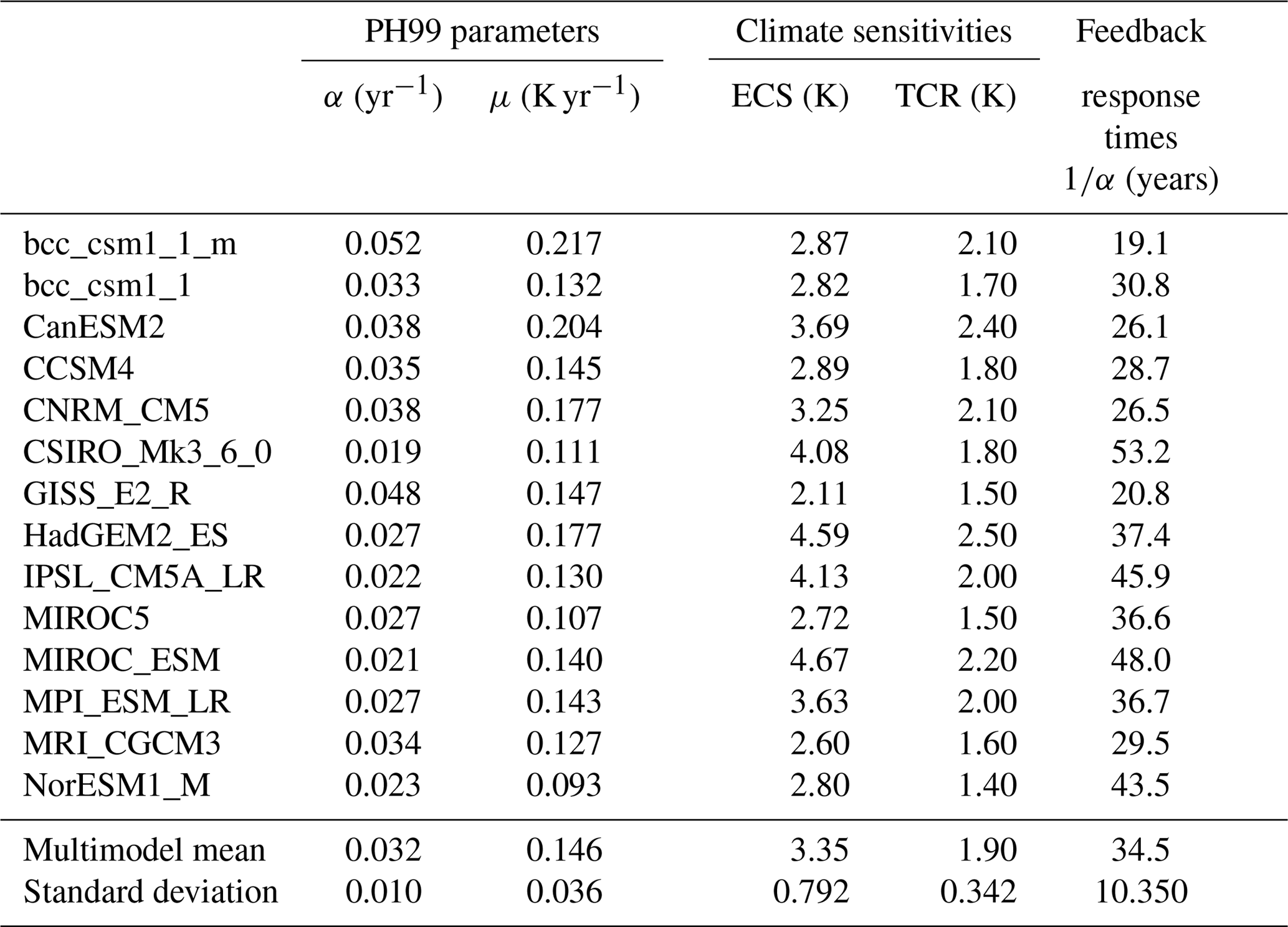
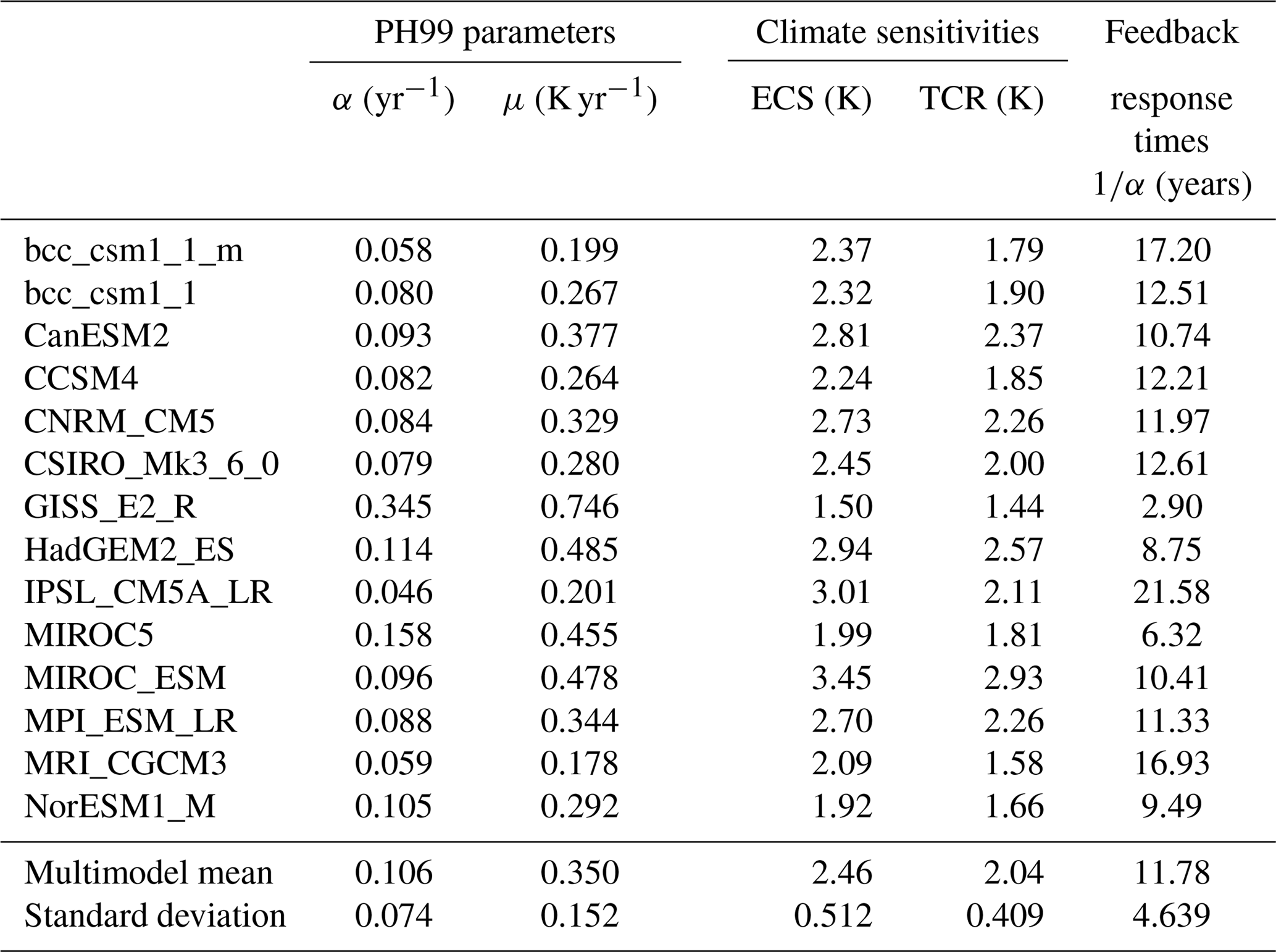
Some difficulty arises due to the fact that AOGCMs have not been run for 2 K-target-compatible scenarios for CO₂-only forcing but solely for a plethora of simultaneous forcings that would add up to a total forcing. Hence we generalize Eq. (1) to its total-forcing counterpart (see Eqs. 4–7) to be driven by total forcing time series as reconstructed in Forster et al. (2013). Accordingly, we utilize scenarios generated by 14 AOGCMs (see Table 1) from CMIP5. From Forster et al. (2013), we also take the ECS and TCR for these 14 models to derive model-specific α and μ, utilizing Eqs. (2) and (3).

Table 1PH99 parameters (α and μ) and feedback response times (1∕α) utilizing data (ECS and TCR) from AOGCMs.

Download Print Version | Download XLSX

In order to generalize Eq. (1), we recall its derivation from an energy balance approach, as summarized in Kriegler and Bruckner (2004), allowing for a physical interpretation of the model. We start by introducing the general energy balance equation, expressing the change in oceanic heat content as the difference of ingoing (F) and outgoing (λT) radiative flux while h denotes the constant effective oceanic heat capacity (see also Geoffroy et al., 2013, Eqs. 1–4).

\begin{matrix} (4) & h \frac{d T}{d t} = F (t) - λ T (t) \end{matrix}

F also represents the total radiative forcing as applied in Forster et al. (2013). However the equation could still not be integrated as h and λ are yet to be determined. In order to solve the posed problem (CO₂-only versus total forcing), we note that h and λ represent universal parameters of PH99 in the sense that their numerical values would not depend on the mix of substances (i.e., CO₂, other greenhouse gases, aerosols) causing the total radiative forcing. Therefore, h and λ can be determined by considering the CO₂-only case and, hence, by tracing them back to the already determined α and μ. For the CO₂-only case, Eq. (4) reads

\begin{matrix} (5) & h \frac{d T}{d t} = - λ T (t) + Q_{2} \frac{\ln c (t)}{\ln 2} . \end{matrix}

Q₂ denotes the additional forcing from the doubling of the CO₂ concentration compared to its preindustrial value and is listed for all of the AOGCMs (see Forster et al., 2013, Table 1).

If we then divide by h, we obtain

\begin{matrix} (6) & \frac{d T}{d t} = - \frac{λ}{h} T (t) + \frac{Q_{2}}{h} \frac{\ln c (t)}{\ln 2} . \end{matrix}

A comparison with Eq. (1) readily reveals

\begin{matrix} (7) & α = \frac{λ}{h} and μ = \frac{Q_{2}}{h \ln 2} . \end{matrix}

These equations would allow for the determination of $h = Q_{2} / (μ \ln 2)$ and λ=αh. Utilizing these equations and Eq. (4), we generate PH99's temperature response to the total radiative forcing as specified in Forster et al. (2013).

The derivation displayed so far can be summarized in terms of the following recipe to generate PH99's parameters on the basis of AOGCMs' ECS and TCR:

set PH99's ECS and TCR equal to the selected AOGCM's ECS and TCR;
numerically invert Eq. (3), right-hand-side expression, to find α (no analytic expression possible);
invert Eq. (2) to find μ;
derive h and λ from Eq. (7), and then utilize Eq. (4), divided by h.

Finally, to avoid differences occurring over the historical period (pre-2006 for the RCPs), we need to initialize PH99 with each AOGCM's 2006 temperature anomaly with respect to the preindustrial value. To do this, for each AOGCM we calculate the mean temperature over the period 1881–1910 and set this as the preindustrial value. We then calculate the mean temperature over the period 1991–2020 and use this as an indicator for the 2006 temperature level. The difference between these two values is fixed as the initial temperature anomaly for PH99.

Each temperature trajectory should be compared to the temperature data from the corresponding AOGCM. As for GMT-target-constrained economic optimizations (Clarke et al., 2014; Edenhofer et al., 2005), the maximum GMT (rather than the whole time series) is of special importance. Hence we use the difference between the respective 2071–2100 GMT time averages of PH99 and the AOGCM as an error metric. If the deviations are tolerable (accurate to within 0.1 K), the climate module is validated; if they are intolerable, we proceed with steps two and three.

2.2 Step two

For each AOGCM, α and μ are tuned such that the difference between PH99 and the AOGCM GMT anomaly for the RCP2.6 scenario in the period 2006–2100 is minimized using a least-squares approach. For further diagnostics we then determine the new “effective” ECS and TCR from Eqs. (2) and (3). As in step one, the deviations in 2071–2100 means of GMT between PH99 and the respective AOGCM are determined as an accuracy check.

2.3 Step three

Lastly, we validate the PH99 model versions generated in step two. For this purpose, independent temperature and forcing paths must be run as a nontrivial test to check whether the trained climate module can accurately project other temperature data trajectories. To do so, the values for α and μ determined in step two are implemented in PH99, the latter then being driven by the total climate forcing of the RCP4.5 and RCP8.5 scenarios. Similar to steps one and two, the deviations in 2071–2100 means of GMT between PH99 and the respective AOGCM are determined as an accuracy check.

One might be interested in seeing if the calibrated module is capable of mimicking other scenarios such as RCP6.0 or if PH99 was calibrated to RCP4.5 or others. Stating that, in general, the procedure outlined above brings about similar results, for the sake of brevity of the main text, we present the respective results in Appendix B.

3 Results

Table 1 shows the calculated α and μ together with the feedback response time 1∕α in step one. For all of the indicators we also compute the mean values and standard deviations of the samples. The mean value of the ECS for GCM data is 3.35 K, with a minimum and maximum of 2.11 and 4.67 K, respectively. The mean value of the timescales is roughly 35 years.

Figure 1 represents the projected PH99 temperature evolution for the scenario RCP2.6 of each GCM in 2006–2100, using the data from Table 1 and RCP2.6's forcings. PH99 clearly overestimates the temperature anomaly for all GCMs, especially over the last 30 years. The absolute values of the deviations of mean temperature over the last 30 years (hereafter MTD) from the AOGCM data are shown in Fig. 2. The MTD ranges from 0.22 K for MRI-CGCM3 to approximately 0.79 K for HadGEM2-ES. On average, the deviations are ca. 0.45 K. This is clearly a large error, in both units of annual GMT standard deviation as well as the climate policy dimension. Accordingly, we must proceed with step two.

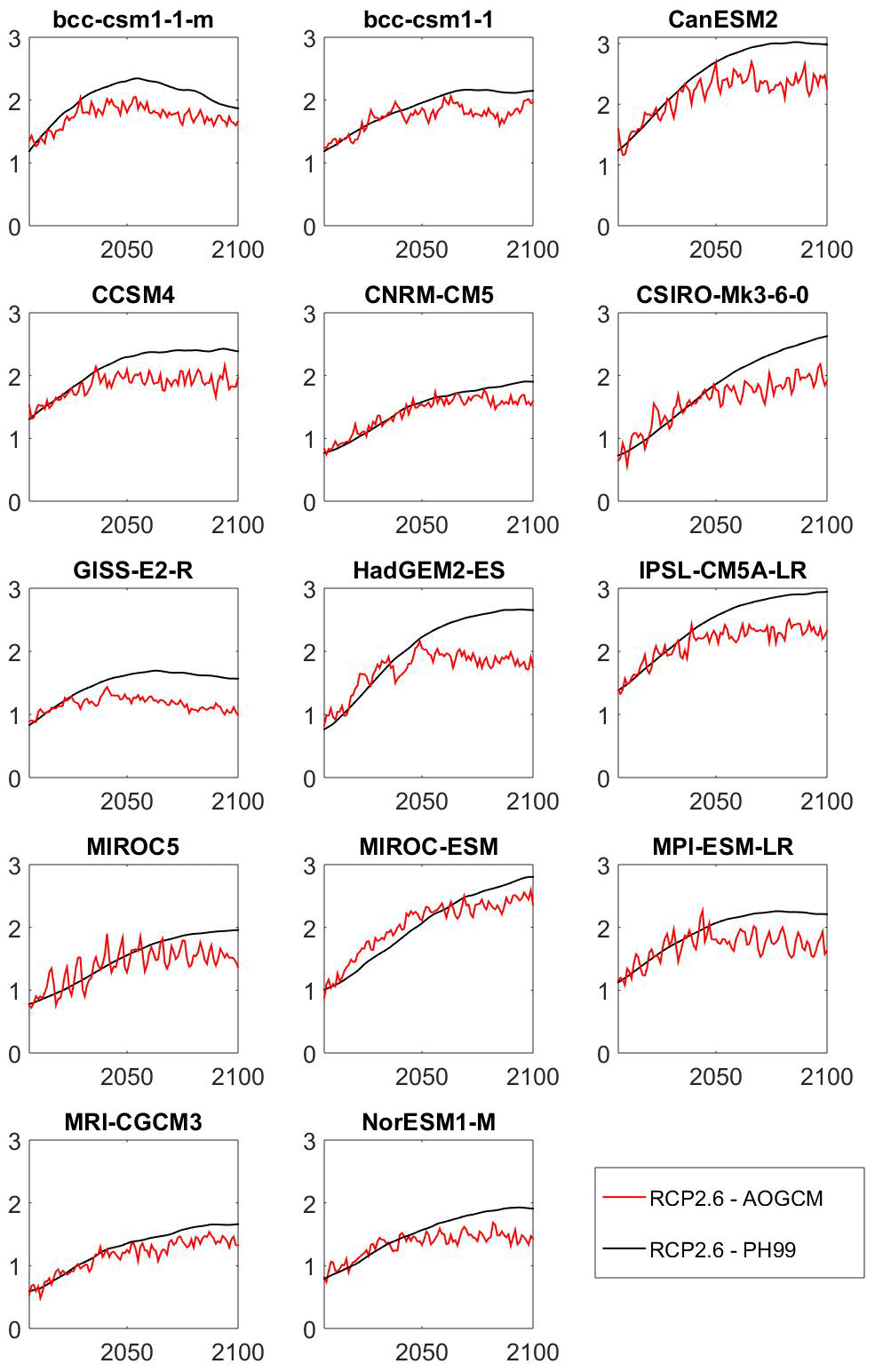
https://www.earth-syst-dynam.net/10/135/2019/esd-10-135-2019-f01

Figure 1Comparison of temperature paths (K) projected by PH99 (black curve), calibrated by an AOGCM's ECS and TCR, to the corresponding AOGCM's temperature paths (red curve). Deviations on the order of 0.5 K for 2100 are observed.

Download

In step two, for each of the GCMs, we tune α and μ such that the GMT deviations for the whole period 2006–2100 are minimized in a least-squares manner as represented in Figs. 3 and 4. From the thereby adjusted α and μ we derive the ECS and TCR, which are presented in Table 2. MTDs for the various AOGCMs are shown in Fig. 2.

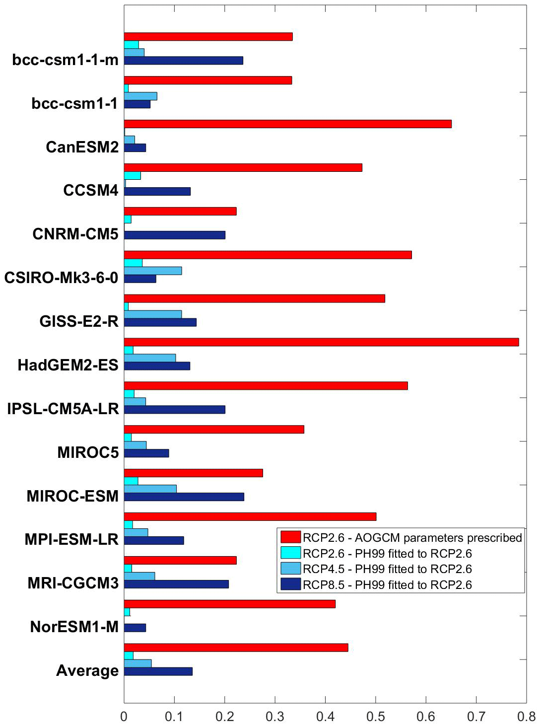
https://www.earth-syst-dynam.net/10/135/2019/esd-10-135-2019-f02

Figure 2Modulus of deviations of GMT (K) mean values of PH99 over the period 2071–2100 from corresponding AOGCM means. The red bars show the deviations for RCP2.6 when α and μ are from Table 1 and not fitted. The cyan bars show the deviations in RCP2.6 when α and μ are fitted to the AOGCM's RCP2.6 data. The light blue bars show the deviations for RCP4.5 when α and μ are kept at their RCP2.6-fitted values (validation). The dark blue bars show the deviations for RCP8.5 when α and μ are kept at their RCP2.6-fitted values (validation).

Download

The results tell us three main things. Firstly, the average of the absolute values of deviations is significantly reduced when α and μ are tuned. Indeed, the MTD average drops to below 0.02 K. Secondly, while the average ECS decreases by 0.9 K (from 3.35 to 2.46 K), the average TCR increases by 0.14 K (from 1.90 to 2.04 K). Thirdly, the mean value of feedback response times decreases significantly, from roughly 35 years to less than 12 years.

For validation we move on to step three. We utilize the RCP4.5 temperature and forcing data as provided by Forster et al. (2013). In Figs. 3 and 4 the respective GMT trajectories for any AOGCM are contrasted with the PH99-generated ones, where α and μ are fixed to their values as determined in step two. The MTDs are shown in Fig. 2. The results confirm that the climate module is sufficiently well trained in the second step that it can suitably mimic the actual temperatures (accurate to within 0.1 K) for RCP4.5 and RCP8.5. As shown, the average MTD is approximately 0.05 K for RCP4.5 and about 0.14 K for RCP8.5. For RCP4.5, the deviations for three of the GCMs, namely CCSM4, CNRM-CM5, and NorESM1-M, are even better than those diagnosed for RCP2.6 in step two. See Appendix B for further analyses.

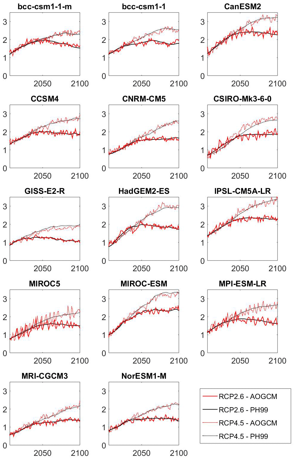
https://www.earth-syst-dynam.net/10/135/2019/esd-10-135-2019-f03

Figure 3Comparison of temperature evolutions (K) projected by the climate module PH99 (solid and dotted black curves) to the actual AOGCM's temperature (solid and dotted red curves). α and μ have been tuned to fit the PH99 temperature path (solid black curve) to the respective AOGCM's RCP2.6 temperature path (solid red curve). Using the fitted α and μ, and taking the forcing reconstructed for RCP4.5 into account, PH99 also reproduces the projected RCP4.5 (dotted black curve). The dotted red curve shows the actual RCP4.5 temperatures.

Download

https://www.earth-syst-dynam.net/10/135/2019/esd-10-135-2019-f04

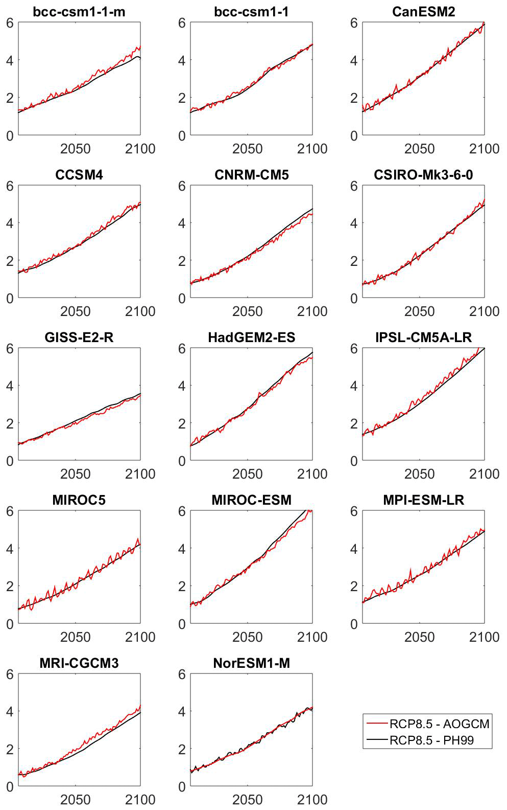
Figure 4Comparison of temperature evolutions (K) projected by the climate module PH99 (black solid curves) in the RCP8.5 scenario to the actual AOGCM's temperature (red solid curves) in the RCP8.5 scenario. α and μ are taken from the second step, in which PH99 is calibrated to the RCP2.6 scenario.

Download

4 A mapping of ECS onto their PH99-specific counterparts α and μ

Finally, we attempt to abstract from fitting PH99 to individual AOGCMs and provide an approximate way to calibrate PH99 within the cloud of AOGCMs simply by knowing the ECS. Then PH99 could be utilized for any ECS in analyses in which the ECS is uncertain.

4.1 An existing mapping for PH99

Before diving into our suggestions, we examine one of the existing options (a reader solely interested in our improved method of utilizing PH99 can move straight on to Sect. 4.2). We inspect the curve suggested by Lorenz et al. (2012), which correlates α and μ to ECS. Using a sample from Frame et al. (2005) and assuming a strict relationship between 1∕μ and ECS, Lorenz et al. (2012) suggest the following approximation:

\begin{matrix} (8) & \frac{1}{μ} \approx \frac{1}{\overline{μ}} - 10 \exp (- 0.5 ECS), \end{matrix}

where $\overline{μ}$ is the mean value of μ in the sample (see Fig. 7 in Lorenz et al., 2012; all quantities measured in the units utilized in Kriegler and Bruckner, 2004). Knowing μ, Eq. (2) is used to determine α. In turn, Eqs. (2) and (8) have been repeatedly used in studies employing MIND and concerning uncertainties and ECS (Neubersch et al., 2014; Roshan et al., 2019; Roth et al., 2015).

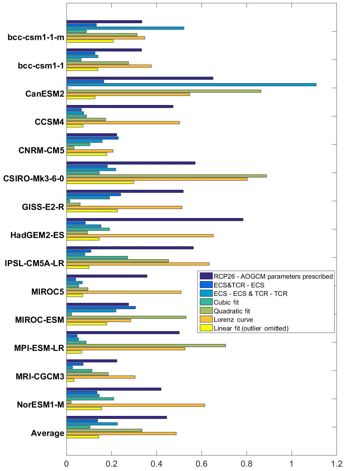
https://www.earth-syst-dynam.net/10/135/2019/esd-10-135-2019-f05

Figure 5Modulus of mean temperature deviations (K) over the period 2071–2100 (MTD) for PH99 from AOGCMs when α, μ, ECS, and TCR from Table 2 are related to ECS and TCR in Table 1. Using linear (yellow bars), quadratic (light green bars), and cubic functions (dark green bars), α and μ are related to ECS when the outlier is put out for the linear case. Using linear fits, ECS and TCR are related to ECS (blue bars). Using linear fits, ECS and TCR are related to ECS and TCR, respectively (light blue bars). The dark blue bars show the deviations for RCP2.6 when α and μ are from Table 1 and not fitted (the same as Fig. 2). The orange bars indicate MTD using Lorenz's curve.

Download

We employ Eqs. (2) and (8) for all ECSs from Table 1 and show the MTDs for the RCP2.6 scenario in Fig. 5. Note that TCR can readily be calculated using Eq. (3). Clearly, on average, employing Lorenz's curve does not result in a better situation than step one. However, this might not necessarily be a case of comparing like with like. At the time of Frame et al. (2005), the two-dimensional uncertainty information was obtained by reconstructing the 20th century's warming signal from fingerprinting by means of a single AOGCM and then using these observational data as a constraint. It is well known that observational constraints may lead to different distributions than ensembles of AOGCMs do (Andrews and Allen, 2008). Nevertheless we include this piece of information here for the sake of completeness.

Table 2PH99 parameters (α and μ), climate sensitivities (ECS and TCR), and feedback response times (1∕α) after fitting PH99 GMT time series to AOGCM RCP2.6 GMT time series.

Download Print Version | Download XLSX

4.2 A multiple AOGCM-based mapping for PH99

Given the inferred estimates in Table 2, one can directly relate α and μ to the ECS. To do so, we generate polynomial fits (of orders of 2 and 3) of α and μ against all AOGCMs' ECSs. Predicting a two-dimensional manifold from ECS alone implicitly exploits the fact that AOGCMs' TCRs can be predicted well using ECSs (see e.g., Meinshausen et al., 2009) in a statistical sense. Another option would be to derive α and μ analytically (like in the first step) when the inferred ECS and TCR are correlated to the ECS and TCR of AOGCMs.

Figure 6 relates α and μ (from Table 2) to the ECS (from Table 1), using linear, quadratic, and cubic polynomial approximations. For the case of a linear approximation, we put the model GISS_E2_R out as an outlier. Figure 5 indicates that on average all approximations mimic the actual temperature paths better than a non-fitted one. The cubic estimation projects significantly smaller deviations compared to the quadratic approximation and slightly smaller deviations compared to the linear approximation. The maximum MTD in the cubic approximation is 0.3 K for IPSL-CM5A-LR, which is roughly a third of the maximum in the quadratic approximation that is revealed for CSIRO-Mk3-6-0.

https://www.earth-syst-dynam.net/10/135/2019/esd-10-135-2019-f06

Figure 6Quadratic (a, b), cubic (c, d), and linear (e, f) relationships of μ (a, c, e) and α (b, d, f) in Table 2 to ECS in Table 1. Notice that in the linear case the model GISS_E2_R, as an outlier, is out.

Download

We also consider alternative ways to map ECS and TCR from the 14 utilized AOGCMs onto PH99-intrinsic properties, going beyond the scheme displayed in Fig. 6. As one option, shown in Fig. 7, we linearly regress the ECS and TCR values inferred from step two against their original AOGCM counterparts and obtain

\begin{matrix} (9) & {ECS}_{PH 99} \approx a {ECS}_{AOGCM} + b, \end{matrix}

with a=0.5846, b=0.5095 K, and R²=0.8158, as long as ECS_PH99 < ECS_AOGCM and

\begin{matrix} (10) & {TCR}_{PH 99} \approx c {TCR}_{AOGCM} + d, \end{matrix}

with c=0.9763, d=0.1829 K, and R²=0.667.

https://www.earth-syst-dynam.net/10/135/2019/esd-10-135-2019-f07

Figure 7Inferred effective TCR (K) vs. AOGCMs' TCR (K) (a), inferred effective ECS (K) vs. AOGCMs' ECS (K) (b), and inferred effective TCR (K) vs. AOGCMs' ECS (K) (c). While the TCRs differ by less than 0.2 K, the ECSs differ by up to 2 K. This opens the door for a discussion as to whether PH99 should be calibrated using scenario-class-adjusted effectively lower ECS values.

Download

The other option consists in using Eq. (9) along with a linearly regressed TCR_PH99 over ECS_AOGCM, that is

\begin{matrix} (11) & {TCR}_{PH 99} \approx m {ECS}_{AOGCM} + n, \end{matrix}

with m=0.4582, n=0.5044 K, and R²=0.7876.

The respective MTDs are shown in Fig. 5. Although both approximations mimic the actual temperature paths better than a non-fitted one, regressing both the inferred effective ECS and TCR solely against AOGCMs' ECS (hereafter ETE) clearly offers the best overall approximation.

Using the ETE has four major advantages over all other options dealt with here, especially for the IAM community. Firstly, its approximation is better than all options but the cubic fit. Secondly the ETE still has an advantage over the cubic fit because one can easily use a broader range of climate sensitivities, for example, from 1 to 9 K, which may not be accurately determined by the cubic fit. Even though the cubic fit may yield a better approximation, in our analysis it is only better by 0.03 K at the expense of a nonintuitive shape that might result in even worse deviations for out-of-sample data. Thirdly, prior knowledge regarding the TCR is no longer a decisive factor. Note that prior knowledge regarding the TCR can make approximations better. However, as we tested, for example, in the case of linearly regressing both the inferred effective ECS and TCR against both AOGCMs' ECS and TCR, the R squares for Eqs. (9) and (11) only improve by 6 % and 7 % respectively, and the MTD is no better than the ETE. Finally, in the case of ETE, we do not need to re-evaluate our sample and possibly drop any model as an outlier. Given the explorations already carried out and their performance, we leave explorations beyond the linear approximation for future research.

5 An analytic interpretation of the AOGCM–PH99 intercomparison

In the following, we explain why PH99 systematically overestimates maximum GMT for peaking scenarios when fitted for exponentially growing scenarios. As an AOGCM is analytically not accessible, we investigate an intermediate step of model replacement by moving from a one-box to a two-box SCM (as utilized in DICE; Nordhaus, 2013). In fact we qualitatively trace back the effects reported so far to the information loss incurred by replacing a two-box SCM with a one-box SCM like PH99. We then also investigate the quality of alternative fitting schemes based on our semi-analytic analysis, which complements our previously mentioned AOGCM-based validation.

Following Geoffroy et al. (2013) we introduce a two-box SCM as a more universal emulator of AOGCMs' mapping from radiative forcing onto temperature.

\begin{array}{l} (12) & C \frac{d T_{2 B}}{d t} = F - λ_{2 B} T_{2 B} - δ (T_{2 B} - T_{0}) \\ (13) & C_{0} \frac{d T_{0}}{d t} = δ (T_{2 B} - T_{0}) \end{array}

T_2B denotes the two-box analogue of the one-box temperature T in Eq. (1). The upper and the lower equations represent the upper and the lower ocean, respectively.

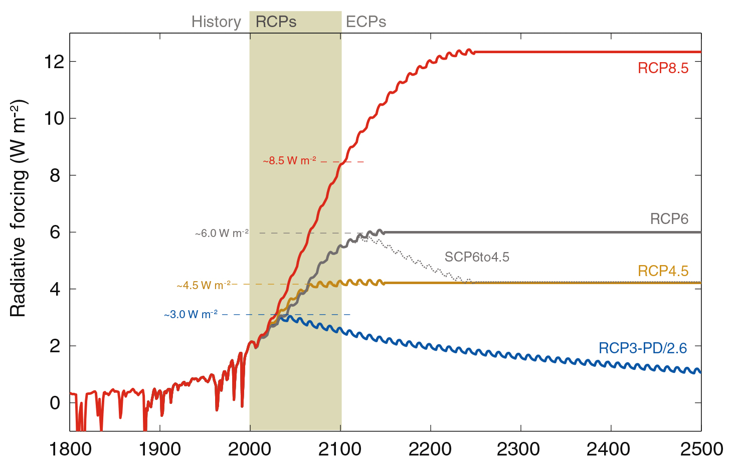
https://www.earth-syst-dynam.net/10/135/2019/esd-10-135-2019-f08

Figure 8Total radiative forcing (anthropogenic plus natural) for RCPs – supporting the original names of the four pathways, as there is a close match among peaking, stabilization, and 2100 levels for RCP2.6 (also called RCP3-PD), RCP4.5 and RCP6, and RCP8.5, respectively (taken from Meinshausen et al., 2011b).

Download

In order to contrast PH99 with this two-box model, we search for analytic approximations of generic shapes of the forcing F(t) and examine the long-term projections under various RCPs as depicted in Meinshausen et al. (2011b) – an excerpt is included in Fig. 8 for the reader's convenience. Particularly in view of the peaking, mitigation-oriented lowest forcing scenario, we approximate forcing paths in three phases: zero forcing, linear increase, and linear decrease, under a continuity assumption.

\begin{matrix} (14) & F (t) = \{\begin{cases} 0 & for t < 0 \\ k_{1} t & for 0 \leq t \leq t_{1} \\ k_{2} (t - t_{1}) + k_{1} t_{1} & for t > t_{1} \end{cases} \end{matrix}

We approximately identify t₁ with the year 2035 and t=0 with 100 years earlier, i.e., we assume a ramp-up time t₁ for the forcing of roughly 100 years. Furthermore, k₂<0 and $| k_{2} / k_{1} | = : ε ≪ 1$ . From Fig. 8 we approximate a generic value of ε=0.2. For $0 \leq t \leq t_{1}$ we draw on Geoffroy et al. (2013 – see their Eq. 14):

\begin{array}{l} T_{2 B} (0 \leq t \leq t_{1}) & = \frac{k_{1}}{λ_{2 B}} (t - τ_{f} a_{f} (1 - e^{- \frac{t}{τ_{f}}}) \\ (15) & - τ_{s} a_{s} (1 - e^{- \frac{t}{τ_{s}}})) . \end{array}

This represents two linear modes of amplitudes a_f and a_s (with a sum equal to 1), delayed by the characteristic timescales of a fast and a slow mode, τ_f and τ_s, respectively, and continuously matched to the initial condition “0” by an exponential. In Geoffroy et al. (2013) the two-box model is fitted to 16 AOGCMs. After having reviewed their results, we can make the following two simplifying assumptions: (i) both amplitudes a_f and a_s approximately equal 1∕2 (see their Fig. 3a – amplitudes range from 0.35 to 0.65) and (ii) τ_f≈0 (values range from 1 to 5.5 years; see their Table 4; for centennial effects, this mode would nearly match the equilibrium response). Furthermore we can see that τ_s ranges from 100 to 300 years for 15 out of 16 AOGCMs. Hence the two-box model is characterized by a marked timescale separation between the two linear modes. With the aid of these two approximations, the last equation can be simplified to

\begin{matrix} (16) & T_{2 B} (0 \leq t \leq t_{1}) \approx \frac{k_{1}}{λ_{2 B}} (t - \frac{τ}{2} (1 - e^{- \frac{t}{τ}})) with τ := τ_{s} . \end{matrix}

We then extend the analytic range of that formula, given the two approximations above, for t>t₁ (for a derivation; see Appendix C):

\begin{array}{l} T_{2 B} (t > t_{1}) & \approx \frac{k_{1}}{λ_{2 B}} (- ε t + (1 + ε) t_{1} \\ (17) & + \frac{τ}{2} (ε + e^{- \frac{t}{τ}} - (1 + ε) e^{- \frac{(t - t_{1})}{τ}})) . \end{array}

The analogous expressions for the one-box model read

\begin{array}{l} T (0 \leq t \leq t_{1}) = & \frac{k_{1}}{λ} (t - θ (1 - e^{- \frac{t}{θ}})), \\ (18) & θ := \frac{1}{α}, λ from Eq . (7), \end{array}

and

\begin{array}{l} T (t > t_{1}) & = \frac{k_{1}}{λ} (- ε (t - θ) + (1 + ε) t_{1} \\ (19) & + θ (e^{- \frac{t}{θ}} - (1 + ε) e^{- \frac{(t - t_{1})}{θ}})) . \end{array}

5.1 Explaining the PH99–AOGCM discrepancy for equal ECS and TCR values

We are now prepared to mimic step one in Sect. 2: we calibrate the one-box model such that it is characterized by the same ECS and TCR as the two-box model. As $λ = Q_{2} / {ECS}_{2 B}$ , equal ECS values for both models deliver λ=λ_2B.

Determining the second degree of freedom of PH99 (e.g., as expressed by θ) from some transient property proves more intricate. We choose

\begin{matrix} (20) & T (t_{TCR}) = T_{2 B} (t_{TCR}), \end{matrix}

where we introduce t_TCR as the moment in time when T needs to be evaluated in order to determine TCR. In Appendix A we note, by definition, that $t_{TCR} = (\ln 2) / γ \approx 70$ years for a growth rate γ=1 % yr⁻¹ of the carbon dioxide concentration; hence $0 < t_{TCR} < t_{1}$ . Therefore, when exploiting Eq. (20), Eqs. (16) and (18) (rather than Eqs. 17 and 19) apply and result in the expression

\begin{matrix} (21) & h (\frac{θ}{t_{TCR}}) = \frac{1}{2} h (\frac{τ}{t_{TCR}}), \end{matrix}

with h denoting the auxiliary function (see Fig. 9)

\begin{matrix} (22) & h (x) := (1 - e^{- \frac{1}{x}}) x, \end{matrix}

where

\begin{matrix} (23) & lim_{x \to 0} h (x) = 0, lim_{x \to \infty} h (x) = 1, h (x) \approx x for x ≪ 1 . \end{matrix}

From this, we can already get a first impression of the scale of θ, prior to numerical inversion: as τ is generically markedly larger than t_TCR, the right-hand side of the defining equation above approximates 1∕2. Further, if we boldly assume a slight timescale separation between θ and t_TCR, the former being smaller than the latter, then the linear approximation of h would apply and $θ \approx t_{TCR} / 2 \approx 35$ years. For a centered value of τ=250 years, this approximation is confirmed in a direct numerical treatment of Eq. (21).

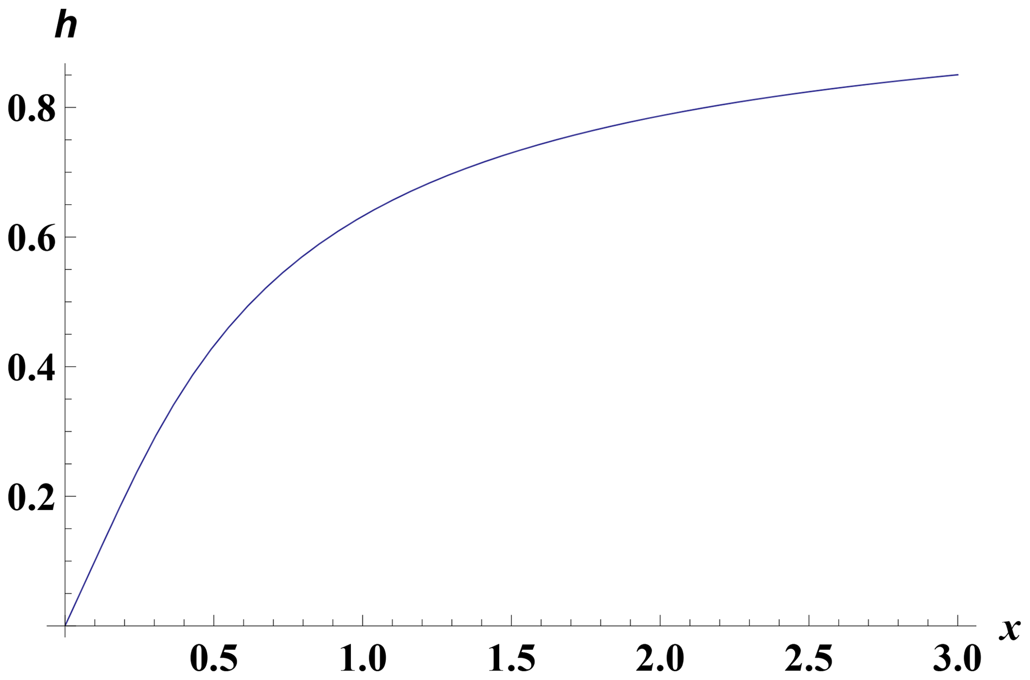
https://www.earth-syst-dynam.net/10/135/2019/esd-10-135-2019-f09

Figure 9The auxiliary function h(x), which links the slow timescale of the two-box model and the timescale of the one-box model.

Download

Hence from the twin timescale separation of “the one-box model mode”, “defining timescale for TCR”, and the “slow mode of the two-box model” we have explained why TCR-oriented fitting exercises of the one-box model would generically result in timescales of roughly 30 to 40 years (see e.g., Anthoff and Tol, 2014; Kriegler and Bruckner, 2004). The factor 1∕2 between the one-box model's timescale and the TCR-defining timescale goes back to the observation of Geoffroy et al. (2013) that the fast and the slow modes both enter the superposition result with approximately equal weights of 1∕2. The slow mode is then too slow to be of much relevance for TCR – a phenomenon not revealed by the one-box model.

We are now equipped to compare the two models' temperature projections and apply the three-phase forcing as defined above for ε=0.2. a₁∕λ is chosen such that peak temperatures enter the 2 K regime for illustrative purposes. We exploit the coincidence that t_TCR just happens to approximately correspond to our starting year 2006 for PH99 (because $2035 - 100 + 70 = 2005$ ). Hence the formulas for the one-box model do not need to be adapted for an explicit initial condition for this purpose. Figure 10 shows that by construction, both temperature responses match at t_TCR≈70 years, although the one-box model's maximum exceeds the maximum by 0.5 K. This phenomenon can be explained as follows. As the one-box model responds with a finite timescale, its derivative must be continuous in response to a continuous forcing. Hence the leading term is quadratic when the forcing starts. In contrast, the two-box model contains a virtually degenerate timescale (the fast one); hence its leading term is linear. If the two curves are to nevertheless match at t_TCR, the one-box model's derivative at t_TCR must transcend the two-box model's derivative. This, together with the right-bending kink in the two-box model's response at t₁, leads to a larger maximum in the one-box model. In summary, on timescales much smaller than the slow mode, the slow mode, compared to the fast mode, cannot develop yet; hence the fast mode will dominate the slow mode. As such, fitting a one-mode model in a convex regime is likely to yield poor predictions of a temperature maximum for mitigation-based forcings.

https://www.earth-syst-dynam.net/10/135/2019/esd-10-135-2019-f10

Figure 10One-box vs. two-box model in response to kink-linear forcing as a stylized interpretation of mitigation-oriented forcing paths and for equal levels of ECS and TCR in both models. Kink-linear curve: two-box model; smooth curve: one-box model. The temperature development of the one-box model overshoots the maximum of the two-box model by roughly 50 %.

Download

This explains the discrepancies found in our PH99–AOGCM comparison when directly transferring AOGCMs' ECS and TCR onto PH99. Figure 10 further suggests that if PH99 were used to predict correct maxima and emulate AOGCMs in this time regime, it would need to be used with a markedly smaller timescale. However, a simple reduction in timescale would lead to a new inter-model discrepancy before the kink; hence the overall amplitude of PH99's response would need to be reduced as well. The latter scales with the ECS. Thus the ECS must be reduced by a certain factor towards a new “effective ECS”, which could also be called a “transient climate sensitivity”.

5.2 Testing the validity of a recalibrated PH99 for a two-box model

In Sect. 5.1 we derived an analytic explanation for why a naïve transfer of an AOGCM's ECS and TCR to PH99 results in a maximum GMT, which is too large when driven by a mitigation forcing scenario. However we show in Sects. 3 and 4 that PH99 in fact is a good emulator of an AOGCM within 0.1 K if it were either directly fitted to that AOGCM or if the AOGCM's ECS and TCR were transformed into effective quantities for PH99. Hereby “good emulator” expresses the fact that the same parameter set can be utilized for any RCP (2.6, 4.5, 6.0, 8.5). From a practical point of view, we could stop our analysis here and suggest that this type of validation might be sufficient to generate trust in PH99 as an emulator for any forcing scenario.

However for further validation, in this subsection we would like to exploit the fact that for a two-box–one-box intercomparison we can validate PH99 for an order of magnitude larger set of forcing scenarios. We systematically test the previously suggested adjustment formulas Eqs. (9) to (11) for a range of t₁ and ε values, hence varying mitigation scenarios, given the alternative ECS and slow mode's timescale τ for the two-box model. We find numerically that θ is on the order of 10 years, and the ECS needs to be reduced by 1∕4 to 1∕3. We test for the centered ECS values of 3 and 4 K and a slow mode's timescale, ranging from 100 to 300 years (see Geoffroy et al., 2013).

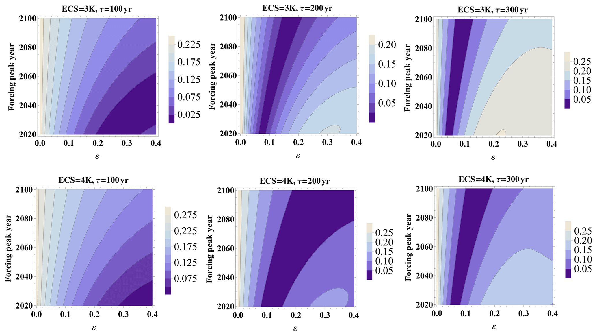
https://www.earth-syst-dynam.net/10/135/2019/esd-10-135-2019-f11

Figure 11Comparing GMT (K) maxima of the two-box model and the one-box model, the latter being adjusted to the former by prescribing the linearly transformed ECS and TCR according to the scheme ETE. Abscissa is ε and ordinate is changed peaking year t₁, transformed to years however, for the two-box ECS of 3 and 4 K, and τ=100, 200, 300 years. The relative error (max. GMT difference normalized by the max. GMT of the two-box model) is markedly smaller than for the case of prior adjustment.

Download

In principle, for any forcing scenario characterized by varying t₁ and ε, we would need to compare GMT as calculated by Eqs. (18) and (19) vs. Eqs. (16) and (17). However all of these equations derive GMT for the boundary condition of zero temperature at t=0. Conversely, our validation scheme as utilized in Sects. 3 and 4 fix PH99 to the AOGCM at the year 2006. The latter point in time we denote by t₀(≈t_TCR). Having transformed ECS and TCR according to Eqs. (9)–(11), we cannot expect that T(t₀)=T_2B(t₀) any longer. Therefore we have to force the solution of PH99 to match the solution of the two-box model at t₀ and call the thereby initialized solution of PH99 “T_init”:

\begin{matrix} (24) & T_{init} (t_{0}) = T_{2 B} (t_{0}) . \end{matrix}

We generate T_init(t) from T(t) (see Eqs. 18 and 19) by adding a suitably scaled solution of the homogenous counterpart of Eq. (4):

\begin{matrix} (25) & T_{init} (t \geq t_{0}) = T (t) + (T_{2 B} (t_{0}) - T (t_{0})) e^{- \frac{(t - t_{0})}{θ}} . \end{matrix}

Figure 11 shows the relative deviations of the GMT maxima of the one-box and the two-box model for the extrapolation scheme ETE (Eqs. 9 and 11). In a certain regime, the extrapolation delivers sufficiently accurate results, however, not everywhere. When utilizing the mapping scheme represented by Eqs. (9) and (10), the results look similar. The overall impression is that the mapping removes the bias. However, it does not deliver a universal correction as found for the direct intercomparison between PH99 and AOGCMs. Hence we cannot exclude the possibility that AOGCMs are easier to emulate as they contain many more timescales than the two-box model and their effects might in part cancel.

While we observe a qualitative gain, Fig. 11 reveals there is still room for improvement. Accordingly, we further transform the ECS to request perfect matching for t₁=100 years, ε=0.2; the results can be seen in Fig. 12. The fit is much further improved such that a major fraction of (t₁, ε) values would lead to a relative error of <5 %, and another large fraction would lead to a relative error of <10 %. As the standard deviation of annual GMT is between 0.1 and 0.2 ^∘C and a typical application might be a cost-effectiveness analysis of the 2 ^∘C target, such errors might still seem tolerable. However we observe structural problems for very small values of ε, the latter implying very late assumption of a maximum. In this case, the slow mode becomes more relevant, and hence the quality of the calibration deteriorates. We find that the calibration is valid for a time horizon on the order of t₁ to 2 t₁, i.e., on the order of the time to peak forcing.

https://www.earth-syst-dynam.net/10/135/2019/esd-10-135-2019-f12

Figure 12Similar to the previous figure (relative max. GMT error with abscissa of ε and ordinate of t₁ in years), however for a further adjusted ECS of the one-box model, such that perfect matching is achieved for t₁=100 years, ε=0.2, and a one-box timescale of 12 years. For most of the parameter settings, the relative error is below 10 %.

Download

6 Discussion

The previous section offers a key mechanism to explain why, for given ECS and TCR, GMT responses generated by PH99 in response to peak-and-decline forcing scenarios are biased towards higher temperatures. How does this relate to the observation that PH99 tends to underestimate the effect of greenhouse gas emissions (van Vuuren et al., 2011a) as mentioned in our introduction? In fact, van Vuuren et al. (2011a) describe a different forcing experiment: a step function (see their Fig. 3). Here FUND, based on PH99, displays a GMT lower than that of MAGICC-4 by more than 0.8 K at certain times during the most transient phase, although both models share the same ECS. This can be explained by the lack of timescales faster than 35 years (the latter characterizing PH99 in standard calibrations) within PH99. Whether PH99 over- or underestimates GMT is hence a strong function of the functional shape of forcing. Our article highlights the effects of naïvely calibrating PH99 when assessing mitigation scenarios.

Additional mechanisms are also possible. Firstly, the statistical errors in determining AOGCMs' ECS, TCR, and Q₂ may lead, mediated through the nonlinear mapping to PH99's parameters, to an overall bias in PH99's GMT. Furthermore, diagnosing the total radiative forcing active in an AOGCM is a complex undertaking (see, e.g., Meinshausen et al., 2011a, for a discussion). A bias to the high end here would also result in inaccurately large GMT responses by PH99.

However, in the context of this article, we contend that the information loss when moving from a two-box to a one-box model is the key source of the observed discrepancy – we find Fig. 10 compelling in this regard. Complying with the latter interpretation raises a key question: can PH99 be seen as a “physical model” and if so, what are the implications for users? It is readily apparent that a one-box model cannot mimic a two-box model, characterized by a marked timescale separation for all forcings at all times. However it is equally clear that the simplest temperature equation is in fact the one that treats the ocean as a single box. It would still explain warming with forcing in a quasi-linear manner, though with some delay. If we are willing to accept that the calibration of PH99 is time horizon specific, then PH99 still holds some semi-physical meaning. If, however, this is seen as unacceptable, then we would have to recognize that PH99 is more an efficient emulator than a physical model. In this context we would like to recall that virtually every model has a limited range of validity – and as such, PH99 is no different from most other models.

When investigating the one-box and two-box models' differences, our research also suggests that within the class of peak-and-decline scenarios PH99 provides a good emulation (accurate to within 0.2 K for a generic AOGCM setting such as ECS = 4 K, a peaking of forcing between 2020 and 2100, and a ratio of slopes of pre- and post-peaking forcing of 0.1 to 0.4). For the AOGCM–PH99 intercomparison, PH99 performs even better: for RCP2.6, RCP4.5, RCP6.0 (∼0.1 K) and approximately 0.2 K for RCP8.5.

What are the ramifications of our findings for previous publications based on PH99? Those authors who claimed to have worked with PH99 in conjunction with ECS = 3 K have effectively worked with a more complex model in conjunction with ECS ≈ 4 K for the centennial time horizon. Much of the work performed based on MIND in conjunction with PH99 and the lognormal distribution for ECS by Wigley and Raper (2001) has essentially been based on a lognormal distribution shifted to larger ECS values. The 5 %, 50 %, and 95 % quantiles of the lognormal distribution by Wigley and Raper (2001) are 1.2, 2.6, and 5.8 K, respectively. When interpreting these values as PH99 values, as they have in fact been utilized in PH99 for the MIND model since Lorenz et al. (2012), in the sense of a rough estimate one could ask what the corresponding effective ECS values of a more complex model according to our Fig. 7 were. The respective values are 1.2, 3.6, and 9.0 K. From Fig. 13, which reflects IPCC AR5's synopsis of current knowledge regarding ECS (Bindoff et al., 2013), we can see that these are still in line with the range spanned by instrumental studies. Hence the results obtained by PH99 in conjunction with the distribution by Wigley and Raper (2001) are not erroneous but simply need to be reinterpreted as rather high-end representatives within the collection of ranges as seen in IPCC AR5.

https://www.earth-syst-dynam.net/10/135/2019/esd-10-135-2019-f13

Figure 13Probability density distributions of ECS according to IPCC AR5 WG-I (Bindoff et al., 2013, Fig. 10.20).

Download

For future applications we can conclude that PH99 must be applied and interpreted with greater care – utilizing transformed values for ECS and TCR – than in the past, if it is not to be replaced by at least a two-box model as suggested by Geoffroy et al. (2013) and implemented in DICE (Nordhaus, 2013). One-box models like PH99 can be crucial for modeling decision-making under uncertainty and anticipated future learning. As an illustration, execution of the MIND model currently demands between hours and days for 20 different values of climate sensitivity in conjunction with one learning step (Elnaz Roshan, personal communication, 2018). The execution time needed will grow exponentially with the number of learning steps and at least linearly with the number of state variables influenced by uncertainty. For endogenous learning in a recursive design, computation time scales factorially with the numerical resolution per state variable. The change from a one-box to a two-box model might hence imply an order of magnitude larger execution time (Christian Traeger, personal communication, 2018, in conjunction with Traeger, 2014). So a one-box model will remain an attractive alternative in numerical applications addressing decision-making under anticipated future learning. Users who would like to go that road might, however, also consider the augmented one-box model by Traeger (2014) as an alternative to PH99, employing an additional exogenous forcing of that single box to somewhat emulate two boxes.

7 Summary and conclusion

We utilize recent data on total radiative forcing (Forster et al., 2013) from 14 state-of-the-art CMIP5 atmosphere ocean general circulation models (AOGCMs) in order to test the validity of the one-box climate module by Petschel-Held et al. (1999, “PH99”) for scenarios approximately compatible with the 2^∘ target. PH99 is currently utilized within the integrated assessment models FUND, MIND, and PAGE.

We find that when prescribing the equilibrium climate sensitivity (ECS) and transient climate response (TCR) of these AOGCMs to the emulator PH99, global mean temperature (GMT) is generically projected 0.5 K higher by PH99 than by the corresponding AOGCM. In contrast, by directly fitting PH99 to the RCP2.6 time series and validating with the RCP4.5 and RCP6.0 series, we find that PH99 can emulate AOGCMs to a degree of accuracy better than 0.1 K. Even for RCP8.5 the error is on the same order of magnitude, although somewhat larger (up to 0.2 K).

We numerically demonstrate that PH99 can be used to excellently emulate AOGCMs (accurate to within 0.1 K on average) within centennial-scale integrated assessment of the 2 K target, provided its ECS and TCR are reinterpreted as effective values and mapped from original ECS and TCR values. We suggest such a mapping.

Furthermore we explain the observed discrepancies and the need to reduce PH99's ECS compared to the AOGCM's ECS as being due to the information loss produced by approximating a two-box-based energy balance model with a one-box-based model. The key point is that PH99 has a fundamentally different response shape to an AOGCM and hence ECS alone does not allow one to easily move between the two. The transformation we propose adjusts PH99's ECS, sacrificing agreement in the long-term response in order to gain agreement in the centennial response (which is useful given it is more often than not the timescale of interest).

In fact the slow mode of the two-box model is so slow that in a climate-policy-relevant context it can unfold only up to a relatively small extent; hence for practical purposes the two-box model's ECS cannot fully develop. Accordingly, adjusting the ECS to lower values also proves to be compatible with reducing PH99's response time. When comparing PH99 and AOGCMs, the match is even better – a phenomenon for which the explanation is beyond the scope of this article.

Hence older work based on PH99, executed within FUND, MIND, and PAGE, may need to be reinterpreted in the sense that a response had been sampled that is higher than that of the corresponding AOGCM. This effect, in turn, proves equivalent to utilizing higher ECS values in the more complex model. Even when having dealt with distributions of ECS as for the MIND model, ECS values reinterpreted in that sense are still within the range outlined by IPCC AR5 (see Fig. 13). Accordingly, we see this reinterpretation as a mere numerical fix. In terms of the underlying physics, we stress that using ECS alone to characterize climate response on a timescale of a few hundred years is fundamentally flawed, given that ECS takes on the order of 1000 years to emerge.

For future work, we propose the following steps: (i) by comparison with more sophisticated, multi-box climate modules it should be tested again whether the effect of a transient climate sensitivity (and TCR) alone could explain our observed PH99–AOGCM discrepancy; (ii) future discussions with the AOGCM community should illuminate to what extent the further explanations we suggested might also apply, thereby potentially reducing the need to correct for PH99; (iii) an AOGCM- and scenario class-independent yet centennial-timescale-specific two-dimensional mapping from ECS and TCR on to ECS and TCR and designed for PH99 should be derived in conjunction with two-dimensional distributions inferred from observations as performed in Frame et al. (2005). The IAM community could then be offered both options for emulation: the one presented here, trained by AOGCMs, and one based on observational data and mediated by more complex SCMs.

In summary, PH99 could continue to be used as the most parsimonious emulator of AOGCMs and is especially efficient for decision-making under climate response uncertainty. However its calibration proves to be much more involved than previously assumed. Future users should carefully consider whether they actually want to use PH99 or whether they prefer a less parsimonious solution.

Data availability

For data sets please contact the corresponding author for Forster et al. (2013).

Appendix A: An analytic expression of TCR in PH99

We rearrange Eq. (1) as

\begin{matrix} (A1) & \dot{T} = μ \ln (c) - α T . \end{matrix}

TCR is defined as the temperature change in response to a 1 % yr⁻¹ increase in CO₂ concentration, starting from preindustrial conditions. Hence the concentration, expressed in units of the preindustrial concentration, reads

\begin{matrix} (A2) & c = \exp (γ t), \end{matrix}

with γ denoting the above rate of change. As Eq. (A1) represents a linear ordinary differential equation with constant coefficients, and the initial temperature anomaly is to vanish, its solution reads

\begin{array}{l} T & = μ γ \exp (- α t) \int t \exp (α t) d t \\ (A3) & = \frac{\exp (- α t) μ γ (1 + \exp (α t) \cdot (- 1 + α t))}{α^{2}} . \end{array}

Temperature should be evaluated at t₂ when the concentration is doubled. t₂ is determined by $c (t_{2}) = 2 \Rightarrow t_{2} = \ln 2 / γ$ . From this and Eq. (A3) we conclude Eq. (3). (In fact we find the same result using an expression provided in Andrews and Allen (2008) when we plug in our expression for t₂ into theirs, which is phrased in terms of ECS.)

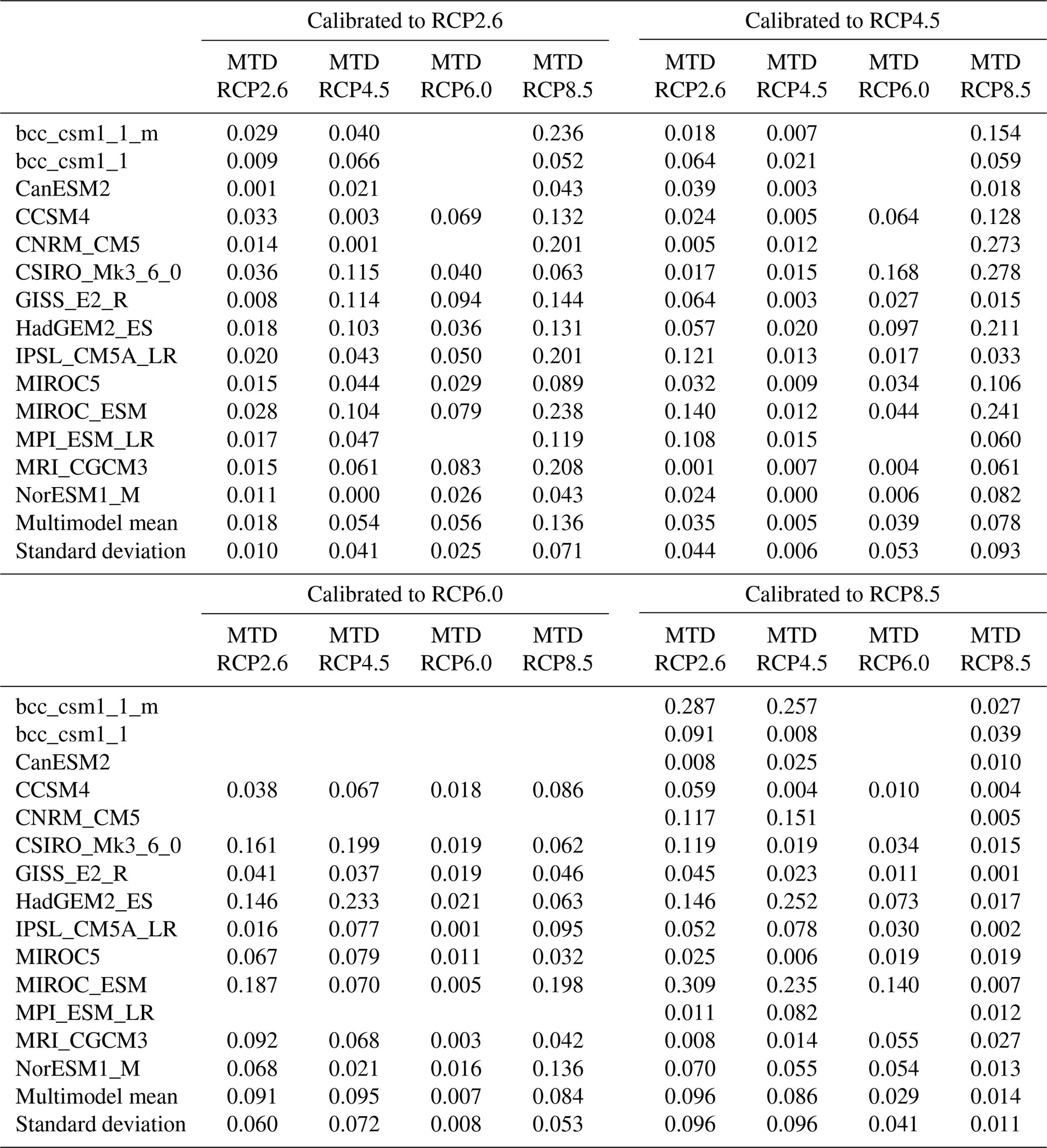
Appendix B: Further analysis on calibration and validation

As further validation of the trained PH99 calibrated to RCP2.6, Fig. B1 shows the respective GMT trajectories of AOGCMs for the RCP6.0 scenario contrasted with its respective PH99-generated ones for which α and μ are fixed to their value as determined in step two. MTDs are shown in the third columns of Table B1. The missing models are due to either lack of temperature trajectories for AOGCM or lack of total forcing. Notice that first, second, and fourth columns are exactly the numbers related to Fig. 2. The results confirm that the climate module is so well trained in the second step that it can appropriately mimic the actual temperatures (accurate to within 0.1 K) for RCP6.0. As shown, the average value of MTD is about 0.06 K for RCP6.0.

Column 5 thereafter in Table B1 shows MTDs in the situations when PH99 is calibrated to the other RCP scenarios and is validated against the others.

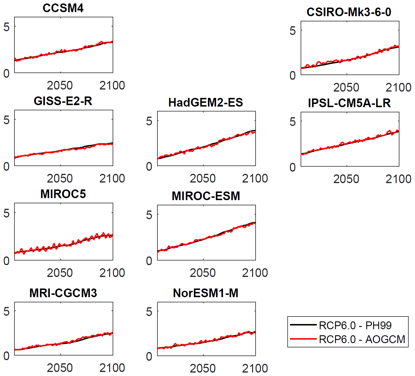
https://www.earth-syst-dynam.net/10/135/2019/esd-10-135-2019-f14

Figure B1The comparison of temperature evolutions projected by the climate module PH99 (black solid curves) in the RCP6.0 scenario to the actual AOGCM's temperature (red solid curves) in the RCP6.0 scenario. α and μ are taken from the second step, in which PH99 is calibrated to the RCP2.6 scenario.

Download

Table B1Modulus of mean temperature deviations over the period 2071–2100 (MTD) for PH99 from the corresponding AOGCM. In the first four columns, PH99 is calibrated to RCP 2.6. In the second four columns, PH99 is calibrated to RCP4.5.

Download Print Version | Download XLSX

Appendix C: Derivation of Eqs. (16)–(18)

We start by rewriting Eq. (15) in a way that it is most consequently decomposed into the contributions from the two modes i∈{f, s} (for “slow” and “fast” modes, respectively).

\begin{matrix} (C1) & T_{2 B} (0 \leq t \leq t_{1}) = \frac{k_{1}}{λ_{2 B}} \sum_{i} a_{i} (t - τ_{i} + τ_{i} e^{- \frac{t}{τ_{i}}}) \end{matrix}

One could derive Eq. (17) from an intuitive perspective by noticing that for any of the modes i, its contribution to the temperature response would consist of an equilibrium response, delayed by τ_i, and a summand of exponential decay that would ensure continuity with respect to the initial condition. This very principle can be followed again for the time horizon beyond t₁.

However, for those readers who would like to see a more formal derivation, we provide the following ansatz: for t>t₁, we decompose T_2B into three contributions, according to the superposition principle for linear differential equations.

T₁ is induced by a forcing k₂(t−t₁) with T₁(t₁)=0. This contribution can be treated analogously to $T_{2 B} (0 < t < t_{1}$ ) when noticing the replacements k₁→k₂, $t \to t - t_{1}$ . From Eq. (C1) we infer
$\begin{matrix} (C2) & T_{1} (t \geq t_{1}) = \frac{k_{2}}{λ_{2 B}} \sum_{i} a_{i} (t - τ_{i} + τ_{i} e^{- \frac{(t - t_{1})}{τ_{i}}}) . \end{matrix}$
T₂ is induced by a constant forcing k₁t₁ with T₂(t₁)=0. This problem has also been solved by Geoffroy et al. (2013) in terms of their Eq. (9), which we rewrite in our notation:
$\begin{matrix} (C3) & T_{2} (t \geq t_{1}) = \frac{k_{1} t_{1}}{λ_{2 B}} \sum_{i} a_{i} (1 - e^{- \frac{(t - t_{1})}{τ_{i}}}) . \end{matrix}$
T₃ is the decaying initial condition at t=t₁. For reasons of continuity, this initial condition is identical to the terminal condition according to Eq. (C1). Hence,
$\begin{matrix} (C4) & T_{3} (t \geq t_{1}) = \frac{k_{1}}{λ_{2 B}} \sum_{i} a_{i} (t_{1} - τ_{i} + τ_{i} e^{- \frac{t_{1}}{τ_{i}}}) e^{- \frac{(t - t_{1})}{τ_{i}}} . \end{matrix}$

When we add these three components, we receive

\begin{array}{l} T_{2 B} (t \geq t_{1}) & = \frac{1}{λ_{2 B}} (\sum_{i} a_{i} (k_{1} t_{1} + k_{2} (t - t_{1} - τ_{i}) \\ (C5) & + e^{- \frac{t}{τ_{i}}} (k_{1} τ_{i} - e^{\frac{t_{1}}{τ_{i}}} (k_{1} - k_{2}) τ_{i}))) . \end{array}

Allowing for the limit τ_f→0 and noticing that $k_{2} = - ε k_{1}$ , we verify Eq. (17) by a summand-by-summand comparison.

Allowing for $τ_{f} = τ_{s} = θ$ (i.e., simulating a one-box setting by a two-box approach), we obtain Eq. (18) from Eq. (C1) and Eq. (19) from Eq. (C5).

Author contributions

MMK performed the statistical analysis. HH provided the analytic analysis. MMK suggested and developed the alternative scheme. Both participated in the writing of the article.

Competing interests

The authors declare that they have no conflicts of interest.

Acknowledgements

The authors would like to thank Jochem Marotzke for drawing their attention to the Forster et al. (2013) article, discussing these results on total forcing and providing the relevant data. In addition, the authors would like to thank Chao Li for supporting the data handling process and making the authors aware of Geoffroy et al. (2013), who discuss negligible AOGCM drift. The authors are also grateful to Elnaz Roshan for her help with the visualizations and providing quantiles of the distribution of Wigley and Raper (2001) on ECS. We thank Matt Fentem for proofreading the second version of our paper from a native speaker's perspective as well as Benjamin Blanz and Manuel Wifling for further proofreading. All remaining errors are ours. Mohammad M. Khabbazan was supported by the Cluster of Excellence “Integrated Climate System Analysis and Prediction” (CliSAP, DFG-EXC177). Finally, the authors would like to thank the three anonymous referees for their valuable criticism and constructive suggestions.

Edited by: Fubao Sun
Reviewed by: three anonymous referees

References

Andrews, D. G. and Allen, M. R.: Diagnosis of climate models in terms of transient climate response and feedback response time, Atmos. Sci. Lett., 9, 7–12, 2008.

Anthoff, D. and Tol, R. S. J.: The Climate Framework for Uncertainty, Negotiation and Distribution (FUND): Technical description, Version 3.6, available at: http://www.fund-model.org (last access: 30 November 2016), 2014.

Bindoff, N. L., Stott, P. A., AchutaRao, K. M., Allen, M. R., Gillett, N., Gutzler, D., Hansingo, K., Hegerl, G., Hu, Y., Jain, S., Mokhov, I. I., Overland, J., Perlwitz, J., Sebbari, R., and Zhang, X.: Detection and Attribution of Climate Change: from Global to Regional, in: Climate Change 2013: The Physical Science Basis, Contribution of Working Group I to the Fifth Assessment Report of the Intergovernmental Panel on Climate Change, edited by: Stocker, T. F., Qin, D., Plattner, G.-K., Tignor, M., Allen, S. K., Boschung, J., Nauels, A., Xia, Y., Bex, V., and Midgley, P. M., Cambridge University Press, Cambridge, UK and New York, NY, USA, 2013.

Bruckner, T., Petschel-Held, G., Leimbach, M., and Toth, F. L.: Methodological aspects of the tolerable windows approach, Climatic Change, 56, 73–89, 2003.

Calel, R. and Stainforth, D. A.: On the Physics of three Integrated Assessment Models, B. Am. Meteorol. Soc., 98, 1199–1216, 2017.

Clarke, L., Jiang, K., Akimoto, K., Babiker, M., Blanford, G., Fisher-Vanden, K., Hourcade, J.-C., Krey, V., Kriegler, E., Löschel, A., McCollum, D., Paltsev, S., Rose, S., Shukla, P. R., Tavoni, M., van der Zwaan, B. C. C., and van Vuuren, D. P.: Assessing Transformation Pathways, in: Climate Change 2014: Mitigation of Climate Change, Contribution of Working Group III to the Fifth Assessment Report of the Intergovernmental Panel on Climate Change, edited by: Edenhofer, O., Pichs-Madruga, R., Sokona, Y., Farahani, E., Kadner, S., Seyboth, K., Adler, A., Baum, I., Brunner, S., Eickemeier, P., Kriemann, B., Savolainen, J., Schlömer, S., von Stechow, C., Zwickel, T., and Minx, J. C., Cambridge University Press, Cambridge, UK and New York, NY, USA, 2014.

Edenhofer, O., Bauer, N., and Kriegler, E.: The impact of technological change on climate protection and welfare: Insights from the model MIND, Ecol. Econ., 54, 277–292, 2005.

Forster, P. M., Andrews, T., Good, P., Gregory, J. M., Jackson, L. S., and Zelinka, M.: Evaluating adjusted forcing and model spread for historical and future scenarios in the CMIP5 generation of climate models, J. Geophys. Res.-Atmos., 118, 1139–1150, https://doi.org/10.1002/jgrd.50174, 2013.

Frame, D. J., Booth, B. B. B., Kettleborough, J. A., Stainforth, D. A., Gregory, J. M., Collins, M., and Allen, M. R.: Constraining climate forecasts: The role of prior assumptions, Geophys. Res. Lett., 32, L09702, https://doi.org/10.1029/2004GL022241, 2005.

Geoffroy, O., Saint-Martin, D., Olivié, D. J. L., Voldoire, A., Bellon, G., and Tytéca, S.: Transient Climate Response in a Two-Layer Energy-Balance Model. Part I: Analytical Solution and Parameter Calibration Using CMIP5 AOGCM Experiments, J. Climate, 26, 1841–1857, https://doi.org/10.1175/JCLI-D-12-00195.1, 2013.

Held, H., Kriegler, E., Lessmann, K., and Edenhofer, O.: Efficient climate policies under technology and climate uncertainty, Energy Econ., 31, S50–S61, 2009.

Hope, C.: The Marginal Impact of CO₂ from PAGE2002: An Integrated Assessment Model Incorporating the IPCC's Five Reasons for Concern, Integrat. Assess. J., 6, 19–56, 2006.

Kattenberg, A., Giorgi, F., Grassl, H., Meehl, G. A., Mitchell, J. F., Stouffer, R. J., Tokioka, T., Weaver, A. J., and Wigley, T. M.: Climate models – projections of future climate, in: Climate Change 1995: The Science of Climate Change, Contribution of Working Group I to the Second Assessment Report of the Intergovernmental Panel on Climate Change, Cambridge University Press, Cambridge, New York, and Melbourne, 285–357, 1996.

Kriegler, E. and Bruckner, T.: Sensitivity analysis of emissions corridors for the 21st century, Climatic Change, 66, 345–387, 2004.

Kunreuther, H., Gupta, S., Bosetti, V., Cooke, R., Dutt, V., Ha-Duong, M., Held, H., Llanes-Regueiro, J., Patt, A., Shittu, E., and Weber, E.: Integrated Risk and Uncertainty Assessment of Climate Change Response Policies, in: Climate Change 2014: Mitigation of Climate Change, Contribution of Working Group III to the Fifth Assessment Report of the Intergovernmental Panel on Climate Change, edited by: Edenhofer, O., Pichs-Madruga, R., Sokona, Y., Farahani, E., Kadner, S., Seyboth, K., Adler, A., Baum, I., Brunner, S., Eickemeier, P., Kriemann, B., Savolainen, J., Schlömer, S., von Stechow, C., Zwickel, T., and Minx, J. C., Cambridge University Press, Cambridge, UK and New York, NY, USA, 2014.

Lorenz, A., Schmidt, M. G. W., Kriegler, E., and Held, H.: Anticipating Climate Threshold Damages, Environ. Model Assess., 17, 163–175, https://doi.org/10.1007/s10666-011-9282-2, 2012.

Luderer, G., Leimbach, M., Bauer, N., and Kriegler, E.: Description of the ReMIND-R model, Potsdam Institute for Climate Impact Research, available at: https://www.pik-potsdam.de/research/sustainable-solutions/models/remind/REMIND_Description.pdf (last access: 30 November 2018), 2011.

Meinshausen, M., Meinshausen, N., Hare, W., Raper, S. C. B., Frieler, K., Knutti, R., Frame, D. J., and Allen, M. R.: Greenhouse-gas emission targets for limiting global warming to 2 ^∘C, Nature, 458, 1158–1162, 2009.

Meinshausen, M., Raper, S. C. B., and Wigley, T. M. L.: Emulating coupled atmosphere–ocean and carbon cycle models with a simpler model, MAGICC6 – Part 1: Model description and calibration, Atmos. Chem. Phys., 11, 1417–1456, https://doi.org/10.5194/acp-11-1417-2011, 2011a.

Meinshausen, M., Smith, S. J., Calvin, K., Daniel, J. S., Kainuma, M. L. T., Lamarque, J.-F., Matsumoto, K., Montzka, S. A., Raper, S. C. B., Riahi, K., Thomson, A., Velders, G. J. M., and van Vuuren, D. P. P.: The RCP greenhouse gas concentrations and their extensions from 1765 to 2300, Climatic Change, 109, 213–214, https://doi.org/10.1007/s10584-011-0156-z, 2011b.

Neubersch, D., Held, H., and Otto, A.: Operationalizing climate targets under learning: An application of cost-risk analysis, Climatic Change, 126, 305–318, 2014.

Nordhaus, W. D.: The climate casino: Risk, uncertainty, and economics for a warming world, Yale University Press, New Haven, USA and London, UK, 2013.

Petschel-Held, G., Schellnhuber, H.-J., Bruckner, T., Toth, F. L., and Hasselmann, K.: The tolerable windows approach: Theoretical and methodological foundations, Climatic Change, 41, 303–331, 1999.

Roshan, E., Khabbazan, M. M., and Held, H.: Cost-Risk Trade-off of Mitigation and Solar Geoengineering – Considering Regional Disparities under Probabilistic Climate Sensitivity, Environ. Resour. Econ., 72, 263–279, 2019.

Roth, R., Neubersch, D., and Held, H.: Evaluating Delayed Climate Policy by Cost-Risk Analysis, EAERE, Helsinki, 24–27 June 2015.

Stankoweit, M., Schmidt, H., Roshan, E., Pieper, P., and Held, H.: Integrated mitigation and solar radiation management scenarios under combined climate guardrails, in: EGU General Assembly Conference Abstracts, 12–17 April 2015, Vienna, Austria, 2015.

Stern, N.: The Stern Review – The Economics of Climate Change, Cambridge, UK, 2007.

Traeger, C.: A 4-Stated DICE: Quantitatively Addressing Uncertainty Effects in Climate Change, Environ. Resour. Econ., 59, 1–37, https://doi.org/10.1007/s10640-014-9776-x, 2014.

UNFCCC: United Nations Framework Convention on Climate Change. Adoption of the Paris Agreement, in: Conference of the Parties on its twenty-first session, 30 November–11 December 2015, Paris, France, 21932, 2016.

van Vuuren, D. P., Lowe, J., Stehfest, E., Gohar, L., Hof, A. F., Hope, C., Warren, R., Meinshausen, M., and Plattner, G.-K.: How well do integrated assessment models simulate climate change?, Climatic Change, 104, 255–285, https://doi.org/10.1007/s10584-009-9764-2, 2011a.

van Vuuren, D. P., Edmonds, J. A., Kainuma, M., Riahi, K., and Weyant, J.: A special issue on the RCPs, Climatic Change, 109, 1–4, https://doi.org/10.1007/s10584-011-0157-y, 2011b.

Wigley, T. M. and Raper, S. C.: Interpretation of high projections for global-mean warming, Science, 293, 451–454, https://doi.org/10.1126/science.1061604, 2001.

Articles

Short summary

We find that for mitigation scenarios, prescribing atmosphere–ocean general circulation models' (AOGCMs') respective equilibrium climate sensitivities (ECSs) and transient climate responses (TCRs) to the one-box model results in too high global mean temperature projections due to the information loss resulting from the reduction of complexity. The one-box model offers a good emulator of these AOGCMs, provided the AOGCM's ECS and TCR values are mapped onto effective one-box counterparts.